1. Introduction

This paper is an extension of work originally presented in  Twelfth International Conference “Management of large-scale system development” (MLSD’2019) [1].

The theory of exchange rate determination is one of the most important components of modern economic theory. Mathematical  models of the medium-term dynamics of the exchange rates are widely presented in the works of classics in [2]-[7], and the monetarist school pay considerable attention to modeling the medium-term and the long-term dynamics of exchange rates. The same can be said about   DSGE-models   in [8].

Medium-term modeling of the exchange rates including the Russian ruble, based on the IFEER-concept (International Flows Equilibrium Exchange Rate concept), was carried out by [9]. This  concept is based on mathematical modeling of the foreign trade operations and the capital flows as the most important macroeconomic fundamental determinants of the exchange rate movements. Several studies (for example, in [10])  consider sources of exchange rate fluctuations in other cases.

Against this background, only a few studies are devoted to the short-term exchange rate dynamics. And first of all, it is necessary to note here the works explained in [11-13].

Mathematical modeling of short-term dynamics will reveal the mechanisms of explosive changes in the exchange rate in crisis periods.

This study will build a new model of the short-term exchange rate dynamics. First of all, we will be interested in the reasons for the deviation from the medium-term equilibrium, and these aspects will be formalized mathematically. But in any case, the basis for mathematical modeling will be the fundamental economic factors that affect the dynamics of the exchange rate. Thus we will use the author’s IFEER-concept and develop it.

2. Conceptual Framework of Exchange Rate Modelling

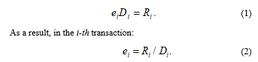
In the basic version, discrete flows are considered in the previous author’s works [9]. For exchange rates that have market pricing, in a certain period we defined in the i-th market transaction:

 – the nominal exchange rate,

 – the volume of the market transaction in the foreign currency,

 – the volume of the market transaction in the national currency.

From  a financial point of view these variables are linked as follows:

However, in this study due to the short-term modeling period author will also apply a differential approach.

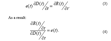
Let’s define R(t) as a streaming continuously differentiated function of funds in the national currency in the foreign exchange market. Accordingly, D(t) is a streaming continuously differentiated function of funds in the foreign currency and  e(t) is the nominal bilateral exchange rate at time t.

By analogy with (1) in the differential form at t:

By analogy with the previously used discrete IFEER-concept [9] we introduce the weight function w(t) for the exchange rate. In the discrete version, the weight function w(i) showed the contribution of the particular i-th transaction, depending on the volume in the foreign currency:

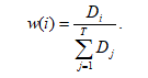In the integral version, the weight function w(t) is also based on the volume of funds in the foreign currency in a certain period T:

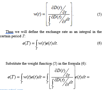
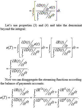
Substitute the weight function (5) in the formula (6):

Let’s use properties (3) and (4) and take the denominator beyond the integral:

Now we can disaggregate the streaming functions according to the balance of payments accounts:

Here funds with the upper index CA belong to the current balance, funds with the upper index K belong to the capital flows balance.

This formula is the main intermediate result of the IFEER-concept, allowing us to identify foreign trade operations and capital flows as  the main factors of the exchange rate movements.

Let’s denote:

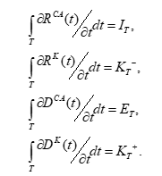From an economic point of view, E_T is the volume of funds as the supply of the foreign currency from export operations, I_T is the demand in the national currency for the foreign currency from import operations.  is the capital outflow as the demand in the national currency for the foreign currency and  is the capital inflow as the supply of the foreign currency.

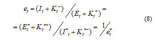
At this conceptual level, the exchange rate dependence has a dynamic form by T:

However, for the two involved parties, the nominal exchange rate is determined symmetrically because the country’s export is another country’s import and the capital outflow is the inflow for the other side.  Here the asterisk shows the financial and economic variables of the opposite counterparty in this two-country world:

It should be noted that the dependence (7) is natural from the economic point of view,  since,  for example,  the increase in demand for imports and an increase in capital outflow leads to an increase in the exchange rate:

The upper sign “-” or “+” here and further on this factor shows that the function respectively strictly decreases or increases.

In terms of partial derivatives, for example:

3. TheTwo-Country Model: TheLevel of theCurrent Account Balance

We will build a two-period model of the exchange rate in periods t and t-1. Since we are going to use point estimates, we will replace the large Т as a period index with the small t for convenience.

Under these conditions formula (7) will take a more decent look, which has already been used by us:

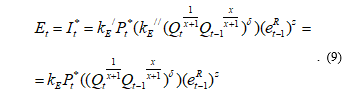
      One of the most important components of the foreign currency inflow to the domestic market is export revenue. However, its level in the period t is determined by decisions of national exporters in the previous period t-1:

here:  is a constant,

 – the aggregate foreign price level,

  – the total domestic real output,

 – the indicator of the international competitive advantages.

The exports of one side in this two-country world are imports of the other side.

 The dependence (9) indicates that only the part of export revenue comes to the domestic currency market. In general, the volume of exports is determined by the part of the total domestic real output  in the foreign prices .

Here intertemporal averaging of the total real output  is used for modeling. Note, that . In this case, the income at t is given more weight than the income at t-1. The method of intertemporal averaging of should not have a significant impact  since it is the least volatile factor.

One of the most important factors of the model is the indicator of the international competitive advantages. This is the real bilateral exchange rate in the previous period t-1:

 Thus, in formula (9) we take into account the possible different degrees of the export functions responses to changes in the indicator of the international competitive advantages and the total domestic real output. For these purposes, we use various adjustable parameters in degrees: . Their relationships will be shown later.

Functional dependence (9) at the same time also has a natural functional character from the economic point of view with respect to the system of the main determinants of the exchange rate:

In accordance with the previous modeling, the demand for the foreign currency from imports is determined completely symmetrically for the other side:

Here:   k_I is a constant,

   – the total foreign real output.

For the purposes of simulation, it is necessary to impose the restrictions: , x=z-y.

      The properties of the stream functions of the current balance operations:

E*=I, I*=E.

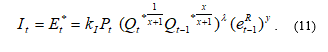
Here it is important to note, that the dependencies (10) and (11) we define for the medium-term environment. But we can assume that these dependencies retain their mathematical factor structure even for the short-term modeling. This is due to the economic inertia of exports and imports in the world economy.

4. TheTwo-Country Model: the Level of the Capital Flows

Of course, the capital flows are one of the most important factors of the exchange rates dynamics. And the developed author’s IFEER-concept allows us to conduct mathematical modeling taking into account the capital flows.

We need to accept the hypotheses about mathematical forms of the basic capital flows dependencies. The capital inflow dependence is an increasing function by the aggregate foreign prices, the indicator of international competitive advantages, and the total domestic real output.

In this context, it is important to note that these functions must be modified for short-term exchange rate modeling in relation to the previously discussed functions in the author’s work [9]. Here the constants k becomes functions by time. For the functional dependence of the capital outflow, for example, it is an increasing function in a crisis period. This shows a short-term increase in capital outflow compared to the medium-term equilibrium dynamics.

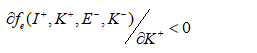
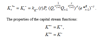
For the capital outflow, thus, the dependence must satisfy the following condition:

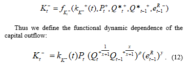The  capital outflow is a part of the domestic product produced in foreign prices.

In the short-term period in the currency market the crisis phenomena lead to a sharp increase in the capital outflow. Mathematically this is expressed in the strict increase function  by t in the dynamic formula (12):

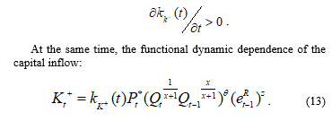Perfectly symmetrical, in the domestic currency market the crisis phenomena leads to a significant reduction of the capital inflows:  a strict decrease of the function by t in the formula (13):

Here  we use the hypotheses about the type of the functions k_К(t), that are not constants for the capital flows in the short-term period.  This distinguishes this model from the previously developed author’s models.

In accordance with the methodology of modeling dependencies are interrelated:

Let’s substitute the functional dependencies (9)-(13) into the basic formula (8):

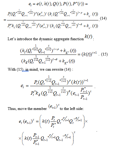
Let’s  make a temporary separation of the modeling variables and re-define and  for convenience:

5. Assessment of Short-Term Dynamic Effects

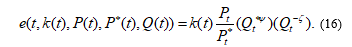
The main result of mathematical modeling is the new nonlinear multi-factor functional dependence of the exchange rate. Here, it should be emphasized that the dynamic functional dependence (16) differs from the previous medium-term dependencies by the type of the dynamic function .

Economically, this function in the short-term period is responsible for explosive changes in the exchange rate dynamics. So, this is the main fundamental difference between this model and the previous author‘s models [9], etc. In those works, these functions are constants in the medium-term in various modifications.

There is significant stability of  in the dynamic functional dependence (15) in comparison with other fundamental factors in the short-term period. So, a strict decrease of the internal function  and a strict increase of the internal function  guarantees us a strict increase of the aggregate function  in a crisis period: . Mathematically this reflects the reasons for the deviation from the medium-term equilibrium.

Direct economic assessment of the short term impact of the function is quite difficult. But we will try to do it using the example of the Russian ruble.

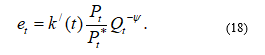
Let’s use the main result of the author‘s work [9]. The medium-term dynamic functional dependence of the exchange rate of the Russian ruble against the US dollar is:

here:  is a constant,

– an estimated parameter.

For  research and verification of this model we used the Russian CPI (Consumer Price Index)  as the model variable P (Federal service of state statistics of Russia), the index of the real Russian GDP as the model variable Q, the prices of blend crude oil as the model variable P* (Intercontinental Exchange, US dollars per brent-mix barrel, Bloomberg information  agency, Bloomberg Terminal).

For  our research the most appropriate  is the crisis period 2013 – 2015. This period is associated with the currency crisis and the significant depreciation of the Russian ruble.

The  ruble/dollar exchange rate (USD/RUR)  is the main rate on the Russian foreign exchange market.  The value of the ruble exchange rate in relation to other world currencies is determined through the cross-rate system.

Thus, as the starting point of the research period, December 2013 was selected. At that time, both the international environment and the domestic macroeconomic situation were stable. The exchange rate of the ruble at that moment was 32,73 USD/RUR according to the Central Bank of Russia.

This study suggests using the least squares method with normalization of the exchange rate values. Since the exchange rate changes quite seriously during crisis periods, it is more important to use relative indicators of changes.

Thus, in accordance with numerical simulation, the solution of the parametric minimization problem

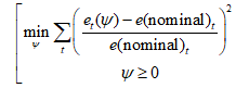is . Here e(nominal) is the nominal exchange rate USD/RUR, according to the Bank of Russia monthly calculations at the end of each period.

       In Figure 1 (monthly data, author’s calculations) we present the dynamics of the exchange rate of the Russian ruble against the US dollar in accordance with the nominal exchange rate e(nominal) and the result dynamic functional dependence of this research e(Theor) (17).

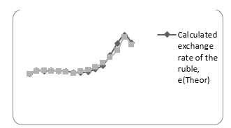Figure 1: The calculated and nominal exchange rates of the Russian ruble  to the US dollar (USD/RUR, monthly data, 2013 – 2015).

The average of absolute normalized deviations of the calculated and nominal exchange rates was 3%, and the average of normalized deviations was 0,3%. As a result, this allows us to conclude that the model quality is high.

This research has shown a high correlation between the exchange rate of the ruble, the inflation, the Russian balance of payments, and other fundamental variables (for example, we can also recommend a work [14]).

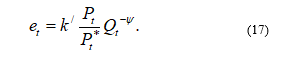
Using the methodology, presented in this paper, and the author’s work [15] (in Russian) it can be shown, that short-term dynamic functional dependence of the exchange rate of the Russian ruble against the US dollar is:

Here, the system of main fundamental economic factors of the exchange rate dynamics in relation to the dependencies (16) and (17) is saved.

In Figure 2 (Moscow Exchange, executions ТОМ) in the period 2013 – 2015solid line represents the medium-term dynamics of the exchange rate of the Russian ruble against the US dollar. We schematically overlaid data from the author’s work [9] and Figure 1. Based on the presented data, we can estimate the cumulative contribution of the function to changes in the ruble exchange rate during crisis periods in the short-term in the amount of 20-25%. The contribution to the crisis period in 2015-2016 can also be estimated at the same amount approximately.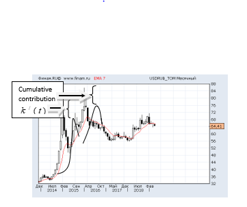Figure 2: USD/RUR quotes

(Moscow Exchange,  monthly data, executions ТОМ, Japanese candlesticks, 2013 – 2018, Information agency *FINAM*)

1. Conclusion

In this study, the new model of short-term exchange rate dynamics was constructed. First of all, we were interested in the reasons for the deviation from the medium-term equilibrium.

The author used the  IFEER-concept as a base and developed it. In this study due to the short-term modeling period, the differential approach was applied. The result was an integrated version of the exchange rate dynamics model. The functional dependencies of the export-import operations and the capital flows were mathematically formalized.

The main result of mathematical modeling is the nonlinear multi-factor dynamic functional dependence of the exchange rate that differs from the previous medium-term functional dependencies by the type of the internal dynamic function. Economically, this function in the short-term period is responsible for explosive changes in the exchange rate dynamics. But in any case, the basis for mathematical modeling was the system of the fundamental economic factors that affect the dynamics of the exchange rate.

The most important limitation of mathematical modeling is the significant difficulty in directly economic assessment of the internal functions  and  that determine short-term capital flows in crisis periods.

But the influence of crisis events on the model in the short term is studied on the Russian financial market at a previous time by assessment of the short-term impact of the function . The  conducted research allowed us to analyze and evaluate the quantitative impact of the short-term effects of the dynamics of the exchange rate of the Russian ruble against the US dollar. The estimated indicators allow us to conclude that the Bank of Russia needs to pursue a more active interventionist policy to maintain the stability of the national currency.

 At the same time, such economic assessments are individual and specific for each currency and each crisis period.

The developed IFEER-concept allows us to model the exchange rate dynamics in other economic conditions. First of all, this concerns the future research of the long-term dynamics of the main world currencies and the Russian ruble.

Conflict of Interest

The author declares no conflict of interest.

1. A. Kuzmin, “Modeling of Short-Term Exchange Rates Dynamics” in Twelfth International Conference “Management of large-scale system development” (MLSD 2019), Publisher: IEEE, 2019, https://doi.org/10.1109/MLSD.2019.8911067
2. R.A. Mundell, “Capital Mobility and Stabilization Under Fixed and Flexible Exchange Rates” Canadian Journal of Economics and Political Science, November, 475-485, 1963. https://doi.org/10.2307/139336
3. A.C. Stockman, “A Theory of Exchange Rate Determination” Journal of Political Economy, August, 88, 673-698, 1980. https://doi.org/10.1086/260897
4. P.B. Clark, R. MacDonald, Exchange Rates and Economic Fundamentals: A Methodological Comparison of BEERs and FEERs, IMF Working Paper 98/67, Washington: International Monetary Fund, March, 1998.
5. P.B. Clark, R. MacDonald, Filtering the BEER a permanent and transitory decomposition, IMF Working Paper 00/144, Washington: International Monetary Fund, 2000.
6. M. Mussa, “The Theory of Exchange Rate Determination” in Exchange Rate Theory and Practice, J.E.O. Bilson, R.C. Marston (eds.), Chicago: University of Chicago Press, NBER, 13-78, 1984.
7. L. Killian, “Exchange Rates and Monetary Fundamentals: What Do We Learn from Long-Horizon Regressions?” Journal of Applied Econometrics, 14( 5), 491-510, 1999. https://doi.org/10.1002/(SICI)1099-1255(199909/10)14:5<491::AID-JAE527>3.0.CO;2-D
8. M. Obstfeld, K. Rogoff, “Exchange Rate Dynamics Redux” Journal of Political Economy, 103 (3), 624-660, 1995. https://doi.org/10.3386/w4693
9. A. Kuzmin, “Exchange Rate of the Ruble Modeling” Advances in Systems Science and Applications, 19(4), 87-93, 2019. https://doi.org/10.25728/assa.2019.19.4.830
10. I. Chowdhury, “Sources of Exchange Rate fluctuation: empirical evidence from six emerging market countries” Applied Financial Economics, 14(1), 697-705, 2004. https://doi.org/10.1080/0960310042000243538
11. R. Dornbush, “Capital Mobility, Flexible Exchange Rate and Macroeconomic Equilibrium” in Recent Developments in International Monetary Economics, E. Claasen, P. Salin (eds.), North-Holland, 261-278, 1976.
12. R. Dornbush, “ Expectations and Exchange Rates Dynamics” Journal of Political Economy, 84, December, 1161-1176, 1976. https://doi.org/10.1086/260506
13. R. Dornbusch, “Equilibrium and Disequilibrium Exchange Rates” Zeitschrift fur Wirtschafts- und Socialwissenschaften, Berlin, 102(6), 573-599, 1982. https://doi.org/10.3386/w0983
14. L. Strizhkova, “The relationship between inflation, exchange rate and parameters of economic policy (on an example of Russia)” Bulletin of the Institute of Economics of the Russian Academy of Sciences, 5, 156-176, 2017. (Article in Russian with an abstract in English)
15. A. Kuzmin, “Modeling short-term dynamics of the ruble exchange rate” Money and credit, 8, 59-65, 2015. (Article in Russian with an abstract in English)

(Click Here)

(Click Here)