1. Introduction

Hypertension or high blood pressure is a disease that can possibly lead to death. Based on the report obtained from the Center of Data and Information, Indonesian Ministry of Health, hypertensive is currently still being a major health concern with a prevalence of 25,8%. On the other hand, the implementation of database technology in the health sector continues to grow rapidly. The amount of data stored in the database is increasing and requires further processing to produce valuable information and knowledge [1] .
The field of science in which data can be processed into knowledge is called data mining. Data mining is a technique that includes a learning process from a machine or computer to automatically analyze and extract knowledge. Classification is one of the basic functions in data mining—a technique that can be used to predict membership of data groups. The process consists of finding a model (or function) that describes and distinguishes classes of data or concepts [2].
Support Vector Machine (SVM) is one method in classification that maps nonlinear input data to several higher dimensional spaces where data can be separated linearly, thus providing a large classification or regression performance [3] .
SVM works based on the principle of Structural Risk Minimization (SRM). SRM in SVM is used to guarantee the upper limit of generalization in the data collection by controlling the capacity (flexibility) of learning outcomes hypothesis [4]. SVM has been used extensively to classify several medical problems, such as diabetes and pre-diabetes classification [5], breast cancer [6] and a heart disease [7] . Based on previous study in liver disease dataset, SVM is known as the classifier compared to naïve bayes.
Meanwhile, problems with unbalanced data are often found due to oversampling which reduces data quality in model construction process. The imbalance of data lies in the unbalanced proportion of the number of categories between independent variables with large difference, thus the majority and minority data class are formed. This condition cause the classification model to be unequal in predicting the minority data class, even though this class still has importance as the object of modeling analysis [8]. Problems are found in the dataset used in this research, where the number of non-hypertensive classes is far greater than the number of hypertensive classes.
Unbalanced data handling needs to be done before modeling stage to develop a classification model with the highest degree of accuracy for all classes. Two techniques to tackle the issue of unbalanced data are Synthetic Minority Oversampling Technique (SMOTE) [9] and Cost Sensitive Learning (CSL) [10]. SMOTE balances the two classes by making systematic data for minority class, while CSL will take into account the impact of misclassification and provide data weighting [8]. This research will cover the performance identification of hypertensive dataset modeling that implements classification method with SMOTE and without SMOTE. The main purpose of this study aims to uncover the significance of oversampling technique implementation for unbalanced data by answering the hypothesis that the combination of the SVM classification method with SMOTE can improve the accuracy of the model.

2. Synthetic Minority Oversampling Technique (SMOTE)

The problem of data imbalance occurs due to a large difference between the number of instances belonging to each data class. Data classes having comparatively more objects are called major classes, while others are called minor classes [11]. The use of unbalanced data in modeling affects the performance of the models obtained. Processing algorithms that ignore data imbalances will tend to be focus too much on major classes and not enough to review minor classes [9]. The Synthetic Minority Oversampling Technique (SMOTE) method is one of the solutions in handling unbalanced data with another different principle from oversampling method that has been previously proposed. Oversampling method focuses on increase random observations, while the SMOTE method increases the amount of minor class data and make it equivalent to the major class by generating new artificial instances [12] .
There are many challenges in dealing with issues of data that are out of balance with the oversampling technique. These problems are related to the addition of random data which can cause overfitting [13]. The SMOTE method is one of the oversampling technique solutions which has the advantage of being successfully applied to various domains as shown in algorithm 1 [14].
Algorithm 1 SMOTE Algorithm
Function SMOTE(T, N, k)
Input : T; N; k ->#minority class examples, Amount of oversampling, #nearest neighbors
Output: (N/100) * T synthetic minority class samples
Variables: Sample [] []: array for original minority class samples;
newindex: keeps a count of number of synthetic samples generated, initialized to 0; Synthetic[][]: array for synthetic samples
if N < 100 then
Randomize the T minority class samples
T = (N/100)*T
N = 100
end if
N = (int)N/100 . -> The amount of SMOTE is assumed to be in integral multiples of 100.
for i = 1 to T do
Compute k nearest neighbors for i, and save the indices in
the nnarray
POPULATE(N, i, nnarray)
end for
end function

Artificial data or synthesis is made based on k-NN algorithm (k-nearest neighbor). The number of k-nearest neighbors is determined by considering the distance between data points of all features. The process of generating artificial data for the numerical data is different from the categorical data. Numerical data are measured by their proximity to Euclidean distance while categorical data are generated based on mode value—the value that appears most often [12]. Calculation of the distance between classes with categorical scale variables is done by the Value Difference Metric (VDM) formula, as follows:

where
∆ (X,Y) : the distance between observations X and Y
w_x w_y : observe weight (negligible)
N : number of explanatory variables
R : worth 1(Manhattan distance) or 2 (Euclidean distance)
δ(x_i,y_i )^r: distance between categories, with the formula:

where
δ(v_1 v_2 ) : distance between V1 and V2
C_1i : number of V1 that belongs to class i
C_2i : number of V2 included in class i
I : number of classes ; i = 1,2,…..,m
C_1 : number of values of 1 occurs
C_2 : number of values of 2 occurs
N : number of categories
K : constants (usually 1)

3. Proposed Research Stages

This research applies a quantitative approach for a case study of hypertensive. Overall, the steps involved consisted of three parts: (1) data pre-processing, (2) building the model and (3) evaluating model performance. The methods used are SVM, ELM, over sampling and under sampling. The performance models are compared with each other. The following are the stages of completing the methodology to be completed.

4. Hypertension Dataset

This research is carried out using a hypertension dataset published in the Kaggle repository sourced from National Health and Nutrition Examination Survey (NHANES) for the year 2008-2016 (https://www.kaggle.com/felmco/nhanes-hypertensive-population-20082016/kernels) with 24435 data rows. A total of 9 features contained in the dataset, as follows:
SEQN,
Gender (Male – 1 and Female – 2),
Age range (from 20 years to 80 years, divided into category 1 to 6),
Race (consists of 1-Mexican American, 2-Other Hispanic, 3-Non-Hispanic White, 4-Non-Hispanic Black, and 5-Other Race),
BMI Range (average body mass index, starting at less than 18,5 kg defined as underweight, normal weight (between 18,5 to 24,9 kg) and overweight(more than 30 kg),
Kidney health condition,
Smoking cigarette or non-smoking,
Diabetes (diabetes, non-diabetes and borderline), and
HPCLASS which has been labeled as class 1 (hypertensive) and class 0 (non-hypertensive).
Samples of all the features in the dataset are shown in Table 1. The dataset will be pre-processed before the modeling.

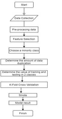Figure: 1. Research Methodology

Table 1. Sample rows from Hypertensive dataset

Seqn	Gen der	Age Range	Ra ce	Bmi Range	Kid ney	Smoke	Dia betes	Hyp class
41475	2	5	5	4	2	2	2	0
41485	2	1	2	3	2	2	2	0
41494	1	2	1	3	2	1	2	0
41516	2	6	3	4	2	1	1	0
41526	2	5	3	3	2	1	2	0
41542	2	4	4	4	2	2	1	0
41550	1	3	1	2	2	1	2	0
41576	1	5	4	4	2	1	1	0
41595	2	6	3	1	2	1	2	0
41612	2	6	3	3	2	2	2	0
41625	2	1	1	4	2	2	2	0
41639	1	2	1	4	2	2	2	0
41674	1	1	4	2	2	2	2	0
41687	1	2	1	2	2	2	2	0
41697	2	1	2	4	2	2	2	0
41711	2	6	3	3	2	2	2	0
41729	1	4	3	4	2	1	2	0

5. Feature Selection

In the pre-processing stage, the selection or extraction of all features of the data is carried out to get the most influential features improve the performance or accuracy of the classification model. Originally, the hypertensive dataset contains of 9 features of the hypertension dataset. The selection implemented by removing a feature “SEQN” in the first column of the dataset which has no effect and only displays the order. The label or class for this dataset is presented in “HYPCLASS” variable.
In the problem of feature selection we wish to minimize equation [15] over σ and α:. The support vector method attempts to find the function from the set f(x, w, b) = w . ϕ(x) + b that minimizes generalization error. We first enlarge the set of functions considered by the algorithm to f(x, w, b, σ) = w . ϕ (x * σ) + b. Note that the mapping ϕ σ(x) = (x * σ) can be represented by choosing the kernel function K in equations. [16]:

for any K . Thus for these kernels the bounds in Theorems still hold. Hence, to minimize T(σ,α) over α and σ we minimize the wrapper functional T_wrap in equation where Talg is given by the equations choosing a fixed value of σ implemented by the kernel. Using equation one minimizes over σ:

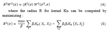
subject ∑_i▒〖β_i=1,β_i ≥ =0,i=1,…,l,and W^2 (α^0,σ)〗 is defined by the maximum of functional using kernel. In a similar way, one can minimize the span bound over σ instead of equation.
Finding the minimum of R^2 W^2over σ requires searching over all possible subsets of n features which is a combinatorial problem. To avoid this problem classical methods of search include greedily adding or removing features (forward or backward selection) and hill climbing. All of these methods are expensive to compute if n is large.
As an alternative to these approaches we suggest the following method: approximate the binary valued vector σ ∈〖{0,1}〗^n with a real valued vector σ ∈ R^n. Then, to find the optimum value of σ one can minimize R^2 W^2, or some other differentiable criterion, by gradient descent. As explained in the derivative of our criterion is:

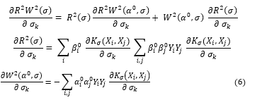
We estimate the minimum of τ(σ,α) by minimizing equation in the space σ∈R^nusing the gradients with the following extra constraint which approximates integer programming.

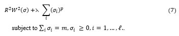
For large enough ⋋ , as p -> 0 only m elements of σ will be nonzero, approximating optimization problem T(σ,α). One can further simplify computations by considering a stepwise approximation procedure to find m features. To do this one can minimize R^2 W^2 (σ) with σ unconstrained. One then sets the q « n smallest values of 0″ to zero, and repeats the minimization until only m nonzero elements of σ remain. This can mean repeatedly training a SVM just a few times, which can be fast.

6. Results

Hypertensive data are classified into hypertensive (1) and non-hypertensive (0) classes. 80% of available data is allocated for training set andremaining 20% for the test set. Data validation is done by the split validation method by dividing three times the test data and three times the training data. Detailed description will be explained in the following subsection.

6.1 Data Visualization

Data visualization is a technique used to communicate data or information in the form of visual objects. In this section, visualization data done by using Python will be displayed in the form of bar graphs. Figure 2 shows the original results of two classifications in hypertension dataset—consists of 7399 hypertensive classes and 17035 non-hypertensive classes. Based on the graph, it can be concluded that the hypertensive class is having comparatively fewer objects than non-hypertensive class.

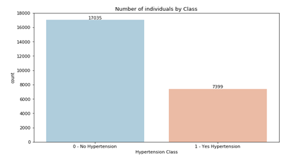Figure.2. Proportion between Hypertensive and Non-Hypertensive

The following graph in Figure 3 shows that the sample of hypertensive patients has greater number in male gender, otherwise non-hypertensive data are dominated with female.

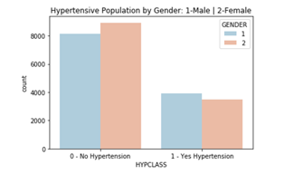Figure 3: Population by gender hypertensive Gender

Figure 4 below shows that the samples of hypertensive and non-hypertensive patients are mostly dominated by the race number 3 (Non-Hispanic White).

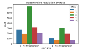Figure 4. Population by Race

6.2 SVM Model and K Fold Cross Validation

The pre-processed data is then used in building the model with the Support Vector Machine (SVM) method. Validation on the SVM classifier model uses the model that has been built with 2 classes of hypertensive and non-hypertensive, in which the value of k = 10 for the K-Fold Cross Validation method. The validation results correspond to the optimal accuracy based on the K-Fold method. Cross Validation rises slightly from initial experiment, where the SVM classifier model has the highest accuracy in the 5th iteration with the highest accuracy value of 95% (average value = 90.2%). The assessment method using the SVM classification method uses the 10-Fold Cross Validation method as presented in Table 1.
Table 2. K Fold Cross Validation with SVM

K-Fold	1	2	3	4	5	6	7	8	9	10	Iteration to	Accuracy Value%
1	1	2	3	4	5	6	7	8	9	10	1	93
2	1	2	3	4	5	6	7	8	9	10	2	90
3	1	2	3	4	5	6	7	8	9	10	3	89
4	1	2	3	4	5	6	7	8	9	10	4	89
5	1	2	3	4	5	6	7	8	9	10	5	95
6	1	2	3	4	5	6	7	8	9	10	6	91
7	1	2	3	4	5	6	7	8	9	10	7	93
8	1	2	3	4	5	6	7	8	9	10	8	87
9	1	2	3	4	5	6	7	8	9	10	9	85
10	1	2	3	4	5	6	7	8	9	10	10	90
Average												90,2

6.3 SMOTE Implementation

Based on the Figure 3 in the previous sub-section, imbalance data are found in hypertensive class (minor class) which is having comparatively fewer objects than non-hypertensive class (major class). In this experiment, oversampling will be carried out on the minority with the Synthetic Minority Over-sampling Technic (SMOTE) method which is a popular method applied in order to deal with cl class ass imbalance. [9]
This technique synthesizes new samples generated from minor class to balance the dataset. New instances of the minor class obtained by forming convex combinations from neighboring instances. Through the number of n_sample = 12000, n_features = 2, n_split = 7 and n_repeats = 4, the accuracy obtained from SVM model is increased to 98%. Figure 5 shows the comparison the value of class 0 (non-hypertensive) and class 1 (hypertensive) after implementing SMOTE method.

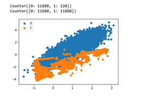Figure.5. Hypertensive dataset experiment with SMOTE

The following is how the SMOTE algorithm works
Step 1: Setting the minority class set A, for each χ ∈A, the k-nearest neighbors of x are obtained by calculating the Euclidean distance between x and every other sample in set A.
Step 2: The sample rate N is set according to the imbalanced proportion. For each χ ∈A , N examples (i.e x1, x2, …xn) are randomly selected from its k-nearest neighbors, and they construct the set A_1.
Step 3: For each example χ_k∈ A_1 (k=1,2,3,…N), the following formula is used to generate a new example:
χ^”= χ+rand (0,1)*|χ-X_k
6.4 Performance of SMOTE and Non-SMOTE Classification Results
Confusion Matrix is used to measure the performance of SVM with SMOTE and SVM performance without SMOTE to classify hypertensive. Then the calculation of accuracy, precision, and recall values is done by calculating the average value of accuracy, precision and recall in each class as shown in Table 3.
Table 3. Results of Comparison of Precision and Recall Values

Class	Non-SMOTE		SMOTE
	SVM Classifier		SVM Classifier
	Precision	Recall	Precision	Recall
Hypertensive	0.88	0.88	0.93	0.85
Non Hypertensive	0.94	0.94	0.88	0.94

Table 4. Average Accuracy Value

Class	Matrix	SVM Classifier
		Non-SMOTE	SMOTE
Hypertensive	Accuracy	91%	98%
Non Hypertensive	Accuracy	91%	98%

From these results, it can be analyzed the effect of SMOTE on the performance of the SVM classification algorithm. The graphic representation of classification model performance result for hypertensive data using SVM classifier with 10-Fold Cross Validation and SMOTE and thus without SMOTE is presented in Figure 6.

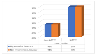Figure 6. Graph Classification Accuracy Results

The results using the combination of SVM and SMOTE, outperformed the SVM classification without SMOTE. The average accuracy based on SVM classifier with SMOTE is higher (98%) compared to SVM classifier without SMOTE (91%).

7. Conclusion

The SVM classification method with a K-Fold Cross Validation resulted on the average of 90.2% of accuracy. SVM is known as a classification method with good prediction results. Based in the experiment conducted in this research, the resulting model is increasing to optimal after running imbalanced dataset using SMOTE with the average of 98% accuracy results.

Acknowledgment

The research publication is fully supported by Bina Nusantara University.

1. M. A. Muslim, S. H. Rukmana, E. Sugiharti, B. Prasetiyo, and S. Alimah, “Optimization of C4.5 algorithm-based particle swarm optimization for breast cancer diagnosis,” J. Phys. Conf. Ser., Figure: 983, (Snik, p. 012063, Mar. 2016. doi :10.1088/1742-6596/983/1/012063.
2. J. P. Jiawei Han, Micheline Kamber, Data mining: Data mining concepts and techniques, 3rd ed. 2012.
3. S. Vijayarani, S. Dhayanand, A. Professor, and M. P. Research Scholar, “Kidney Disease Prediction Using Svm and Ann Algorithms,” Int. J. Comput. Bus. Res. 6(2), 2229–6166, 2015.
4. R. D. F. Adhitia, “Penilaian Esai Jawaban Bahasa Indonesia Menggunakan Metode SVM – LSA Dengan Fitur Generik,” 5(1) 2009. doi:10.21609/jsi.v5i1.260.
5. W. Yu, T. Liu, R. Valdez, M. Gwinn, and M. J. Khoury, “Application of support vector machine modeling for prediction of common diseases: The case of diabetes and pre-diabetes,” BMC Med. Inform. Decis. Mak., 2010. DOI: 10.1186/1472-6947-10-16.
6. I. Maglogiannis, E. Zafiropoulos, and I. Anagnostopoulos, “An intelligent system for automated breast cancer diagnosis and prognosis using SVM based classifiers,” Appl. Intell., 1, 24–36, 2009. DOI: 10.1007/s10489-007-0073-z.
7. M. T., D. Mukherji, N. Padalia, and A. Naidu, “A Heart Disease Prediction Model using SVM-Decision Trees-Logistic Regression (SDL),” Int. J. Comput. Appl., 16, 11–15, 2013. doi: 10.5120/11662-7250.
8. D. Adiangga, “Perbandingan Multivariate Adaptive Regression Spline (MARS) dan Pohon Klasifikasi C5.0 pada Data Tidak Seimbang (Studi Kasus: Pekerja Anak di Jakarta),” 2015.
9. N. V. Chawla, K. W. Bowyer, and L. O. Hall, “SMOTE: Synthetic Minority Over-sampling Technique,” Ecol. Appl., 30(2), 321–357, 2002, DOI: https://doi.org/10.1613/jair.953.
10. C. Elkan, “The Foundations of Cost-Sensitive Learning,” 2001.
11. I. D. Rosi Azmatul, “Penerapan Synthetic Minority Oversampling Technique (Smote) Terhadap Data Tidak Seimbang Pada Pembuatan Model Komposisi Jamu,” Xplore J. Stat., 1, 2013, doi:10.29244/xplore.v1i1.12424.
12. S. Cost and S. Salzberg, “A weighted nearest neighbor algorithm for learning with symbolic features,” Mach. Learn., 10(1), 57–78, 1993, doi:10.1023/A:1022664626993.
13. M. Galar, A. Fern, E. Barrenechea, and H. Bustince, “Hybrid-Based Approaches,” 2012. DOI: 10.1109/TSMCC.2011.2161285.
14. A. Fernandez, S. Garcia, F. Herrera, and N.V. Chawla, “SMOTE for Learning from Imbalanced Data: Progress and Challenges, Marking the 15-year Anniversary,” J. Artif. Intell. Res., 61, 863–905, 2018.
15. U. Alon et al., “Broad patterns of gene expression revealed by clustering analysis of tumor and normal colon tissues probed by oligonucleotide arrays,” Proc. Natl. Acad. Sci. U. S. A., 96(12), 6745–6750, 1999, DOI: 10.1073/pnas.96.12.6745.
16. J. Weston, S. Mukherjee, O. Chapelle, M. Pontil, T. Poggio, and V. Vapnik, “Feature selection for SVMs,” Adv. Neural Inf. Process. Syst., 2001.

(Click Here)

(Click Here)