1. Introduction

The most common type of industrial controller currently is the PID controller. About 90% of the controllers in commercial operation use the PID algorithm. The reason for such a high popularity is the simplicity of construction and industrial use, clarity of operation, suitability for solving most practical problems and low cost. However, the existing methods for calculating the parameters of PID controllers are oriented to linear systems, since the controller itself is a linear dynamic link. If the control object is essentially non-linear, then it is difficult to achieve a good quality of management.

A fuzzy logical controller (FLC) is a controller that contains in its structure a block of fuzzy logic inference. Usually FLC are included in series with the object controls, like traditional controllers [1], [2].

The classical theory of automatic control is focused mainly on the synthesis of linear controllers based on linearized models, however, all real objects are nonlinear. The nonlinearity of the mathematical model is expressed in the presence of static and dynamic nonlinear blocks, such as “saturation”, “dry friction”, “hysteresis”, etc. FLC, which are nonlinear in nature, can control linear objects are better than classic controls, and also manage substantially non-linear objects for which linear controllers cannot provide acceptable quality.

The main problem of using FLC is the need to formalize the control law in the form of fuzzy rules that use linguistic variables for descriptions of inputs and outputs of the controller. First FLC used the experience of an expert to describe the law of control [3], [4], but this method suitable only for a limited range of tasks. Standard options for describing FLC rules rely on the analysis of the phase plane of the object management [5]. FLC step-by-step tuning methods similar to the Ziegler-Nichols method for proportional-integral-differential (PID) controllers [6]. But in general, the task FLC settings is an optimization task, to solve which is enough accurate computer model of the object and powerful global search algorithm [7], [8]. The task is to find a suboptimal solution, satisfying user. In [9], an RBF network is used, which serves to change the coefficients PID controller. Setup is done using genetic algorithm (GA).

Search engine optimization algorithms are subject-independent, the success of their application for setting up FLC depends on the choice of the optimality criterion and the method of describing the controller parameters. This work is devoted to the consideration of solutions to these problems.

2. Solution methods

Experience in designing industrial control systems shows that the behavior of many real dynamic systems can be approximated using the transfer functions of the first or second order (possibly with delay). This feature has led to the widespread adoption of PID controllers as a simple and reliable means of automation. The PID controller equation has the form

Often, options are used only from two terms (1) – proportional differential (PD) and proportional-integral (PI) controllers. In this case, a clear geometric interpretation of the control law is possible, since here the control surface is a plane (figure 1).

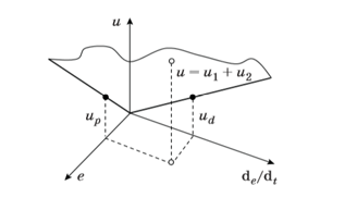Figure 1. Scheme of the control surface of the PD controller

A fuzzy PID-type controller receives the same input signals as a linear PID-controller, but the control law here is described not by a hyperplane, but by some hypersurface. The classical approach to building FLC leads to the use of control rules with three premises (figure 2, where N and DN are normalization and denormalization coefficients).

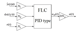Figure 2. The scheme of the fuzzy PID-type controller with three inputs

The above path is inefficient, because when using  terms to describe each input,  control rules are obtained. Using fuzzy controllers, PD- and PI-type two signals are received at the input. It can be shown that if we consider at the output of the PI-type FLC not the value of the output signal , but its increment , then the PI-type FLC control law describes the same rules that the PD-type FLC uses.

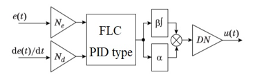Figure 3. Scheme of a simplified description of PID-type FLC

This allows you to use the structure shown in figure 3 to implement PID-type FLC (where  and  are unknown coefficients).

This representation is often used in practice, the number of fuzzy rules here is reduced to . Further simplification of the PID-type FLC description is possible when writing the fuzzy control law in a form similar to (1):

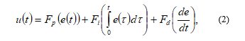where , , and  – some nonlinear functions.

When using  terms to describe each input, only  control rules are required here (figure 4).

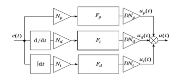Figure 4. PID-type FLC decomposition scheme

Normalization coefficients are selected based on a priori data about the control system. Considering the problem of PID-type FLC synthesis as a task of improving the quality of the PID controller, the following algorithm can be used to select denormalization coefficients [10], [11]:

• A linear PID controller is being synthesized, the parameters of which , , will play the role of denormalization coefficients.
• Non-linear functional dependencies are described that describe the fuzzy control law for each of the input variables.

Thus, in the first step, the basic gain factors are obtained, and in the second step, additional gain factors that are nonlinearly dependent on the input signal.

3. Evolutionary synthesis of nonlinear control law

The search for nonlinear dependencies in (2) can be solved in various ways, however, the most effective here is the use of population metaheuristic methods like genetic algorithm or particle swarm method [12].

The use of a genetic algorithm involves encoding the parameters of a problem using chromosomes whose constituent parts (genes) correspond to individual parameters. A set of chromosomes form a population that evolves over time. The goal of evolution is to improve suitability of chromosomes describing quality solutions to the problem.

The particle swarm method considers individual task parameters as search space coordinates. For each point, the value of the objective function is calculated. A swarm of particles moves in the search space in the direction extremum.

When using both algorithms, the complexity of the task is determined by the number of tunable parameters and the type of objective function.

To describe nonlinear functions ,  and , you can use different methods, in particular, neural RBF networks.

Neural RBF network is a two-layer, it contains a layer of radial basis neurons and a linear output layer [13].

As the radial basis function  commonly used gaussian function

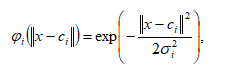where – width of the “window” of the activation function; -the center of the activation RBF function of the -th neuron; -is the input signal.

The output of the RBF network is described by the expression

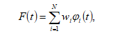where -the weight of the neuron of the output layer.

Nonlinearity ,  and  are positive, i.e. the product of any input signal and corresponding output positively. Therefore, each neuron of the RBF layer has a paired neuron in which the center has the same module, but a different sign. This allows to reduce the number of customizable options.

Thus, each neuron has two parameters, and the third parameter is the output weight of the neuron.

The optimization problem can be simplified if one pre-distributes RBF neurons to the base scale and select a fixed width of activation functions. Obviously, this operation corresponds to the linguistic description of the input variable using a set of terms (figure 5).

Figure 5. Approximation of static nonlinearity using an RBF network

You can also consider piecewise linear approximation of a nonlinear function. This option can be represented in the form of an RBF network in which radial basis neurons have rectangular activation functions, and the weights of the output layer correspond to the gain of linear sections.

In fact, this means replacing the linear controllers to many linear controllers, each of which is responsible for its own area input space.

Denoting the gain of each linear section as , we get a vector of custom parameters .

Description of the objective function is convenient to perform using a reference model that describes the specified transient requirements. Objective function should evaluate proximity object outputs and a reference model, for example:

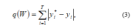where – number of time points during transition process;  and  – are the real and desired output value of the object.

General evolutionary optimization scheme PID-type FLC is shown in figure 6.

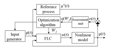Figure 6. Evolutionary optimization of a fuzzy controller

The optimization algorithm cyclically launches an input generator that produces a test exposure to . Each time the controller is started, it gets the parameters  that matches chromosome genetic algorithm or particle coordinates (particle swarm method). At the end transient parameter set gets suitability rating . Then the population (swarm) is converted, and new testing happens. The criterion for ending the process is usually prolonged lack of improvements or exhaustion of the number of given iterations.

A convenient tool for implementing the described approach is the MatLab package with the extensions Simulink and GAtool [14].

4. Implementation examples

The mathematical description of many industrial facilities (electrical, electromechanical, hydraulic, etc.) with one input and one output can be presented in the form of models containing a static non-linear link and a dynamic linear part in series [15], [16].

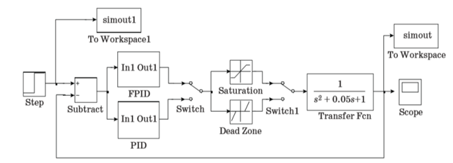Figure 7. Block diagram of the experiment in MatLab Simulink

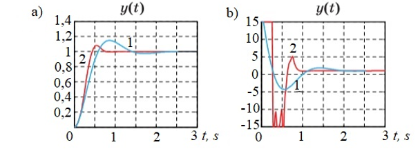Figure 8. Transient graphs (a) and control signal (b) in a system with non-linearity “saturation”: 1 – linear PID controller; 2 – non-linear PID-type FLC

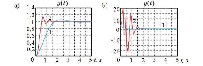Figure 9. Transient graphs (a) and control signal (b) in a system with non-linearity “dead zone”: 1 – linear PID controller; 2 – non-linear PID-type FLC

Nonlinearity of the “saturation” type is introduced into the model to take into account the limitations of variable levels when studying the behavior of control systems in large deviations from the equilibrium position, and also to describe the maximum levels of the control signal.

A non-linear element of the type “dead zone” takes into account the real properties of sensors of actuators and other devices with small input signals. The computational experiment diagram is shown in figure 7.

The control object is an oscillating link, to the input of which nonlinearities and a controller of the selected type can be connected. When setting up the PID controller and PID type FLC, a genetic algorithm was used. The simout blocks were used to compute (3).

The simulation results for an object with non-linearity “saturation” are presented in figure 8 a and b, and for an object with non-linearity “dead zone” – in figure 9 a and b. As follows from figure 8 a and 9 a, the transition process time was reduced by about half, although at the same time the energy costs of management increase (see figure 8 b and 9 b).

Nonlinear functions describing the fuzzy control law for each PID-type FLC channel obtained as a result of genetic training are shown in figure 10. The resulting functions ,  and  turned out to be significantly different for objects with different nonlinearities. This result is predictable, since the controller can be considered as an inverse model of the object.

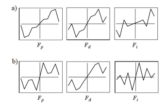Figure 10. Graphs of functions — nonlinear mappings over three FLC channels, obtained for an object with the characteristic “saturation” (a) and “dead band” (b)

5. Conclusion

Thus, the article considers a two-step algorithm for the evolutionary synthesis of PID-type FLC, which, in the first step, optimizes the gain of the linear PID controller, and in the second step, additional gain, nonlinearly dependent on the input signal. A comparative analysis of the simulation results shows that the use of PID-type FLC can significantly improve the parameters of the transition process. The proposed technique is simple and can be recommended for use in numerous technical applications to improve the operation of linear PID controllers.

Conflict of Interest

The authors declare no conflict of interest.

Acknowledgment

This research received no specific grant from any funding agency in the public, commercial or not-for-profit sectors.

1. K. Passino, S. Yurkovich, “Fuzzy Control”, Addison-Wesley, NJ, 522 p. 1998. https://www2.ece.ohio-state.edu/~passino/FCbook.pdf.
2. D. Rutkovskaya, M. Pilinskiy, L. Rutkovskiy, Neyronnie seti, geneticheskie algoritmi i nechetkie sistemi- M.: Goryachaya liniya-Telekom, 452 p. 2006. https://www.twirpx.com/file/1934241/.
3. E.H. Mamdani, S. Assilian, “An Experiment in Linguistic Synthesis with Fuzzy Logic Controller”, Int. J. Man-Machine Studies, 7(1), 1-13. 1975. https://doi.org/10.1016/S0020-7373(75)80002-2.
4. L.P. Holmblad, J.J. Osregaard, “Control of Cement Kiln by Fuzzy Logic. In: Approximate Reasoning in Decision Analysis”, Eds. Amsterdam, New York, Oxford, 389–400, 1982.
5. P.J. Macvicar-Whelan, Fuzzy Sets for Man-Machine Interaction. Int. J. Man-Mach. Studies, 8, 687– 697, 1976.
6. I.X. Siddikov, D.M. Umurzakova, D.B. Yadgarova, Structural-Parametric Synthesis of an Adaptive Fuzzy-Logical System // Universal Journal of Electrical and Electronic Engineering, 7(2), 94-102. 2020. https://DOI: 10.13189/ujeee.2020.070204.
7. V.A. Demchenko, Automation and modeling of technological processes at nuclear power plants and thermal power plants / V. A. Demchenko. – Odessa: Astroprint, – 308 p. 2001. https://www.twirpx.com/file/249124/.
8. O. Cordon, F. Herrera, F. Hoffmann, L. Magdalena, Genetic Fuzzy Systems: Evolutionary Tuning and learning of Fuzzy Knowledge Bases. Sinqgapore, New Jersey, London, Hong Kong, World Scientific Publishing, 462 p. 2001. https://DOI:10.1142/4177.
9. S. Zeng, H. Hu, L Xu, G Li, Nonlinear Adaptive PID Control for Greenhouse Environment Based on RBF Network // Sensors 12, 5328-5348, 2012. https:// DOI: 10.3390/s120505328.
10. K.J. Astrom, “Revisiting the Ziegler-Nichols step response method for PID control”, Journal of Process Control, 4, 635-650, 2004. https://doi:10.1016/j.jprocont.2004.01.002.
11. C. Lu, C. Hsu, C. Juang, “Coordinated control of flexible AC transmission system devices using an evolutionary fuzzy lead-lag controller with advanced continuous ant colony optimization”, IEEE Transactions on Power Systems. 28(1), 385–392, 2013. https://DOI: 10.1109/TPWRS.2012.2206410.
12. X.S. Yang, Engineering Optimization: An Introduc tion with Metaheuristic Applications. — Hoboken: John Wiley & Sons, — 347 p. https://www.academia.edu/457294/Engineering_Optimization_An_Introduction_with_Metaheuristic_Applications, 2010.
13. D. Pelusi, R. Mascella, “Optimal control algorithms for second order systems”, Journal of Computer Science. 9(2), 183–197, 2013. https://doi.org/10.3844/jcssp.2013.183.197.
14. I.X. Siddikov, D.M. Umurzakova, “Mathematical Modeling of Transient Processes of the Automatic Control System of Water Level in the Steam Generator”, Universal Journal of Mechanical Engineering, 7(4): 139-146, 2019. https:// doi: 10.13189/ujme.2019.070401.
15. I.X. Siddikov, D.M. Umurzakova, H.A. Bakhrieva, Adaptive system of fuzzy-logical regulation by temperature mode of a drum boiler // IIUM Engineering Journal, 21(1), 185-192, 2020. https://doi.org/10.31436/iiumej.v21i1.1220.
16. I.X. Siddikov, D.M. Umurzakova, “Neuro-fuzzy Adaptive Control system for Discrete Dynamic Objects. International conference on information science and communications technologies applications, trends and opportunities”, (ICISCT 2019). Tashkent University of information technologies named after Muhammad al-Khwarizmi. –Tashkent. 4-6 November, 2019. https://DOI: 10.1109/ICISCT47635.2019.9012027.

(Click Here)

(Click Here)