1. Introduction

This paper is an extension of work that was originally presented in ISSE 2019 conference [1]. Originally, paper [1] focused on creation of a multi-body model for analyzing the vibro-acoustic characters inside the eBike. The current work illustrates the extension of the previous setups to the optimization domain using the finite element techniques.

In the current pedelec industry, the core problems faced by manufacturers are the structural behaviors, such as vibration and deformation, due to loading. Lately, researchers have mainly focused on the development of the electric motors, batteries and power electronics, which has laid a solid foundation for building advanced electric powertrains [2]-[4]. Improving the energy efficiency of the entire electromechanical drives was the essential parameter, while areas related to vehicle dynamics and structural properties, such as vibration, noise, stiffness, compliance, etc., are not extensively examined. However, several findings show that the vibrations of electric drives can lead to several problems in regard to stability and driving comfort of the vehicle [5, 6]. In addition, the presence of stresses in structures beyond the yield limits leads to larger deflections and thereby reduce the efficiency of the components [7]. Understanding the static and dynamic behavior of the electromechanical drives therefore remains an essential task for the Original Equipment Manufacturers (OEMs). This paper attempts to develop a method that can be used to capture structural behavior early in the product to avoid unnecessary costs in the later stages of the product lifecycle. The method was developed largely with the help of the Finite Element Modeling techniques (FEM).

The numerical discretization of known structures is a popular topic in computational mechanics. The end user uses the software iteratively to optimize a structure. It is up to him/her to improve the design in order to identify a good geometry [8]. In contrast, topology optimization software outputs the optimal geometry using structured mesh, directly after the optimization task has been defined. Structural topology optimization helps the designer in modeling the type of structure which best fits to satisfy the operating conditions for the problem [9]. It changes the general component layout to find designs with goals such as minimization compliance or maximization of natural frequencies. Stress and compliance optimization are key indicators in the structural design for a range of engineering applications. Optimization helps in the design of mechanical components with lower stress concentrations [10]. Once the results are extracted from the optimization module, they are enhanced using the smoothing functions provided by the optimization tool. It can be seen as a procedure to optimize the rational arrangement of the available elements in the design volume and to eliminate the unnecessary elements.

In a similar way, the structure borne emission from housings must also be optimized. Vibrations are undesirable movements in the powertrain and are responsible for the problematic noise and energy losses in the system. In general, they are generated from excitations at structural components and would later affect the overall performance of the Drive Unit (DU). In order to maintain the efficiency of the drive, vibration and noise emission should be reduced below the threshold values. One way of achieving this is through the dynamic optimization technique [11]. As part of this approach, the simulation template is created to analyze the surface acceleration and acoustic quantities. Later, a dynamic optimization module is developed to strengthen the structure and reduce the vibrations in the drivetrain.

2. State of the Art

2.1. Stress Analysis in Drivetrain Components

 Structural analysis is generally performed to check the durability of certain parts for a particular load and support condition. For the component to be structurally safe, stresses in the body should not be more than the yield strength of the material. Considering the possibility of fatigue failure, the component must be optimized such that the Von-mises stress generated does not exceed the endurance strength of the material. There are several articles that generally describe the stress and deformation of various components such as gears, motors, etc. For instance, paper [12] written by Mao discusses the importance of transmission error in gears and its influence in powertrain structures. Similarly, Chung published his results in paper [13] that focused on stress analysis of helical gears and their deformation profile for different load cases in normal drive trains. Electromechanical drives have distinct structural characteristics. Most of these papers principally illustrate the gear forces in static load cases or influences in the performance of normal drivetrains due to errors at the gears. However, there are no proper references available for analyzing electromechanical drives as entire unit, for example, considering the influences of multiple domains such as axial and electromagnetic forces, static and linear dynamic cases together, or the impact of excitations, forces at the bearings and the structural behavior of the housing combined. Moreover, adding optimization tasks makes the existing scenario more complex. This paper tries to solve this problem by examining and simulating each juncture responsible for deformations, critical stresses etc. In this way, a holistic simulation template is provided with which the entire drivetrain can be analyzed and a future variant with optimized properties can be developed.

2.2. Modal Analysis of Complex Structures

Vibrations are nothing but mechanical oscillations of a system/component at an equilibrium point. A statically balanced object oscillates at a certain frequency depending on its properties such as mass and stiffness. This frequency is referred to as the natural frequency of that structure [14]. The calculation of these frequencies and their respective mode shapes is essential for researchers to understand the vibro-acoustic properties of the components. There are usually two sets of models used to analyze the vibrations of structures, continuous and discrete. The continuous models are mathematical models applied to continuous data and are represented by the Partial Differential Equations (PDE). The coefficients of these PDE’s depend on the geometrical and material properties. Solutions to these equations are obtained using numerical methods such as Dunkerley’s method, Rayleigh-Ritz method, Newton–Raphson method, Galerkin approach, etc., [15 – 17]. The discrete models are those models with finite degrees of freedom and are generally described by ordinary differential equations. Two main techniques that deal with the discrete models are finite element and rigid element methods.

The structure of the DU is complex and consists of more than 60 components and 800000 Degrees Of Freedom (DOF), which makes it difficult to analyze either with the continuous models or the rigid element method. FEM is used as a simulation technique considering the factors such as complexity (large number of DOF’s), modeling (more flexibility to include the effects like contact, hybrid modeling, etc.), adaptability and accuracy (better precision) for calculating the vibrations. FEM generates the physical response of the system at any given position, including some that may have been neglected in an analytical approach. In addition, FEM has an advantage of modeling noise using acoustic finite, infinite elements and the impedance boundaries [18]. The Eigen forms are calculated using the solution technique described by Grimes, Lewis, and Simon in paper [19].

2.3. Relevance of Optimization

Researchers have developed numerous solutions with regard to the structural topology optimization problems. Below is a list of few approaches developed within the topology optimization domain [8]:

• Ground structure approach discussed in the Shiehin’s paper [20].
• Homogenization method described by the Bendsoe and Suzukiin in papers [11, 21], respectively.
• Bubble method shown by the Eschenauer’s paper [9].
• Fully stressed design technique depicted in Xiein’s paper [10].

The first three approaches listed above have some characteristics in common. These are optimization methods with an objective function and a set of design variables and design constraints. They solve the optimization problem, either by a sequential, quadratic programming algorithm (approach 1) or by an optimality criterion concept (approaches 2 and 3). In contrast, the fully stressed design technique, although not an optimization algorithm in the conventional sense, proceeds by removing inefficient material and thereby optimizes the use of the remaining material in the structure, in a step-by-step process.

Within this paper, the methods majorly from approach 1 are used as guidelines for the design of drivetrain structures to improve the stiffness, dynamic characteristics and to reduce the weight of the components. In addition, the optimization design can be regarded as the topology optimization problem of continuum structures. Structural optimization attempts to find the best path for transferring all types of loads.

This paper deals with the optimization of drivetrain structures for both static and dynamic load cases. Using a topology optimization approach to design new drivetrains should take less time than the traditional trial-and-error experiments.

2.4. Definition of the Optimization Task

Optimization can be used to shorten the development phase by upgrading insight and intuition of the designers through an automated process. To optimize the powertrain model, the variable that needs to be optimized must first be determined. Optimizations to minimize stress or to maximize the Eigen frequency are simply not sufficient. The task must be more specific, for example minimizing the maximum node stresses that occur during a static load case with a limitation of the existing weight, or similarly maximizing the sum of the first natural frequencies with limit on volume of the components. The goal of the optimization task is referred to as the objective function. In addition, certain conditions can be enforced during the optimization, for instance, the displacement of a given node can be curtailed to a certain value. This enforced condition is often called a constraint.

In addition, the structural domain called the reference domain can be divided into the design and non-design areas. The non-design domain includes key regions such as supports, boundaries and areas where loads are applied. Therefore, these regions cannot be modified throughout the entire optimization process. With the constraint on weight, objective functions, such as optimizing stress, stiffness, etc., are used for the optimization of the static load case. In linear dynamic analysis, the visco-elastic material definitions are used to simulate the drivetrain. Here, the goal of optimization is to curtail the surface vibrations and acoustic noise below the limits.

Overall an optimization task is represented using three characteristics. Below is a list of the characteristics, including concerning questions:

• Design variables – How can the structure be modified? Values, such as frequencies, weight, volume and stiffness, can be altered to obtain better vibrations.
• Design constraints – Which restrictions must be implemented in the model? Variables, such as mass and volume, can be limited to certain ranges.
• Design objective functions – What should be minimized, maximized, optimized, etc.? Function of compliance with a goal in increasing the stiffness and reducing the stress. Function of natural frequencies (variable) to push the critical spectrum domains, thereby avoiding vibrations.

2.5. Mathematical formulations

2.5.1. Gearmesh Excitations

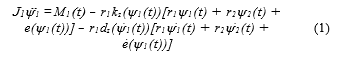
The parametric formulation for gears characterized as lumped mass is shown in (1) (1 – gear1, 2 –gear2). It represents the dynamic Equation of Motion (EOM) of one of the gear with to gearmesh excitations. Here the term e(ψ(t)) includes the effects of parametric excitation. It is developed as sum of mean excitation plus sine curves (considering the harmonics of the tooth cycle) with corresponding amplitudes. ψ_i(t) (i = 1, i = 2 – gear2) and its time derivatives represent the rotation angle, angular velocity and angular acceleration respectively. M, J, r, z, ψ, e, k_z and d_z represent torque, inertia, radius of pitch circle, number of tooth, rotation angle, excitation, stiffness and damping respectively [1].

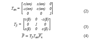
Furthermore, the gear forces are described in (2), (3) and (4). Here,  consists of three components, namely the tangential, radial and axial force of the gear. , , , c and s describe the normal force, rotation matrix for the helix angle, rotation matrix for the normal pressure angle, cosine angle and sine angle, respectively [1]. These gear forces cause the shafts and bearings to vibrate, which in turn sets the structure borne emission in rest structures.

2.5.2. Fluid Structure Coupling

The housing-air coupling occurs at the interface at which the acoustic medium interacts with the structure. This is called the fluid structure interface. This coupling between the housing structure and air medium is modeled by conservation of linear momentum.

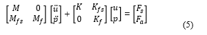
Equation (5) shows the general formulation of the housing and surrounding fluid at its interface. The terms u, M, ,  K, , and  indicate the displacement of housing, mass of the housing, mass of the fluid/ air, mass of the fluid structure interface, stiffness of the structure, stiffness matrix of fluid, stiffness matrix of fluid structure interface, force applied by the structure and force exerted by the air respectively. Detailed information about the coupling finite element models can be found in papers [22, 23].

2.5.3. Optimization formulations

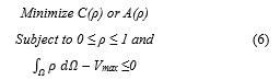
Furthermore, (6) represents the mathematical form of the optimization task. The objectives are defined as minimizing the compliance (C) and the surface accelerations (A). Volume is considered as a design constraint (in this example) and is limited to V_max. ρ is a density vector containing the element densities ρ_e. When ρ_e is 1 we consider an element to be filled whereas an element with ρ_e as 0 is considered to be a void element.  is considered as the design volume of the optimization task. The volume constraint prevents the optimized structure from ending with the full design volume when searching for its maximum structural stiffness.

One way to maximize a structure’s global stiffness is to minimize its compliance. The compliance is therefore defined as the equivalent strain energy of the FE solution, which yields higher stiffness when minimized. The compliance is defined in (7) and u is obtained by solving the equilibrium equation (8).

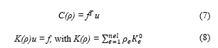   is the initial elemental stiffness matrix. Using the gradient based approach, derivatives with respect to C(ρ) are evaluated. Finally, the case of multiple loads as (9) can be included in the structural optimization task by using weights and objectives that are subjected to a particular load case with the index k. M is the total amount of load cases. Equations (7) and (8) can also be further modified for dynamic optimization of surface accelerations [24].

In previous models, optimality criterion, a controller based algorithm was utilized for the optimization. This is faster than the sensitivity based algorithm since no gradient information is required [11, 24]. However, the controller based algorithm is based on stresses and is limited to optimizing stiffness under a volume fraction constraint. Sensitivities are not evaluated since the controller uses strain energy and stresses as an input. In this paper, the optimization tasks are executed using sensitivity based Method of Moving Asymptotes (MMA) approach. It solves non-linear optimization problems in the sense that it uses sequences with sub-problems that are approximations of the original problem [25]. For MMA, these sub-problems are constructed by gradient information and it is also assumed that these approximations are convex. Different design responses can also be combined, for example if the objective is to minimize compliance, both the volume and effective stress can be included as constraints.

The primary focus of the paper lies in the development and optimization of a three stage transmission. The modeling and simulation section describes the architectural layout, intricacies involved in the development of the static simulation template, the forces in the linear dynamic step, coupling between the vibration and acoustic domains, etc., are described. In the optimization section, housing weights are used as design variables. The vehicle performance and indicators, such as compliance, acoustic pressure, etc., are considered as design objectives.

The design procedure is defined in three steps. First, the FE model is used to analyze the original structure. The stiffness and Von-mises stress obtained from the analysis are then treated as the design variables in the topology optimization. The constraint of the optimization task is the reduction in total mass while improving the performance parameter such as vibration in comparison to the original. Eventually, two different optimized variants are developed: one for the static scenario and the other for the linear dynamic load case.

3. Development of the Numerical Model

Before the optimization task is illustrated, it is essential to create a simulation template that takes into account all the characteristics, such as excitation mechanisms, loads at the bearings, deformations of the critical components, etc. Considering the necessary complexities within the modeling technique enables the user to build a model that is close to reality. Detailed information regarding the simulation templates with analyses at multiple domains, such as the Lumped Parameter Model (LPM), Multi-Body Dynamics (MBD), etc., can be found in papers [1, 23].

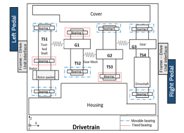Figure 1: Architectural layout of housings, gears, toothed shafts and bearings of the drivetrain

Figure 1 describes the layout of simulated drivetrain instance to check for critical stresses, deformations and Eigen frequencies. The rotation of the toothed shafts and gears would cause transmission errors that lead to vibrations in the structure. The torque at the toothed shafts and axial load at the bearings would in turn cause the housing structures to deform. Along with the load, boundaries are also applied in the simulation template. For instance, the DOF of bearing nodes are either fixed, thus the z-axis rotation is free, or movable, thus the z-axis translation and rotation are free. Furthermore, the drivetrain is connected to pedals at the frame bracket interface; depending on the load case scenario, the model is enforced with loads at the left pedal, right pedal, shaft axles, gear toothmesh, etc.

Vibrations are influenced by structures having heavier mass or greater stiffness. Therefore, the components that contribute to the drive train vibrations must first be determined. Table 1 describes the scaled masses, Young’s modulus and the yield limits of different structures available in the drivetrain. Together, these structures represent about 92 % of the total mass of the power unit. Hence, the structural validation of these components individually and in combination would help to understand the deformations and vibrations of the entire drivetrain in later stages.

The FE software Abaqus and the optimization tool Tosca from Dassault Systems are used to implement the simulation and optimization models [26].

Table 1: Modeling information of the individual components of the drivetrain (scaled)

Component	Mass (Kg)	Young’s modulus (Mpa)	Plasticity limit (MPa)
Housing	0.113	0.119	0.14
Cover	0.077	0.119	0.14
Stator	0.268	0.952	0.651
TS4	0.065	0.938	1
G3	0.063	1	1
TS3	0.065	1	1
G2	0.019	1	1
TS2	0.01	1	1
G1	0.015	1	1
TS1	0.023	1	1
Driveshaft	0.044	0.933	0.94
Rotor packet	0.079	0.881	0.417
Frames	0.045	1	0.515

3.1. Static Analysis Template

This section describes the model parameters associated with simulation of the static load case. It illustrates a simulation template for analyzing the electromechanical drive for its stresses and deformations. In this scenario, the load is applied in multiple steps: first at the left pedal and later at the right pedal.

To test the mechanical strength of the power unit, it must be viewed in its most critical state, i.e., when it is subjected to the maximum forces during its use. For this reason, the bike is considered at a position with a maximum force of 1800 N on the pedals. According to the German standard DIN EN ISO 4210-8 for “bicycles-safety-technical requirements for bicycles”, two cases have to be considered in order to validate the strength of a system [27]. These cases are called” uphill” and ”downhill”.

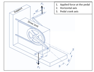Figure 2: Schematic view of the static load case

Figure 2 corresponds to the uphill load case, where the force on the left and right pedals act in the downward and upward directions, respectively. This standard defines the position of the pedals in relation to the axis of the chain, as well as the forces and boundary conditions acting on them.

Furthermore, the Abaqus simulation model developed must comply with these standards. The boundary conditions apply to the chain and frame. In the uphill position, the simulation consists of two steps, in which a force of 1800 N is applied first to the right pedal and then to the left pedal. The mesh is then created and refined so that the simulation converges and areas with high stress are re-meshed finely for better accuracy. Table 2 describes the general information regarding the FE model.

Table 2: FE model information for static load case

Count of nodes	Count of elements	Load step 1	Load step 2
872148	525712	Right pedal 1800 N	Left pedal -1800N

A specific magnesium alloy with a yield limit of 140 MPa is used as the material for the housing structures. The fracture occurs at a plastic elongation of more than 6 %. With a safety factor of 2, the limit value at 3 % is considered further for the simulations.

The maximum stresses of both uphill and downhill simulation are comparable for their respective cases and hence do not allow the most critical case to be determined. In order to circumvent this problem, a life cycle study is performed to determine the most critical position. This is not the subject of this paper, but is carried out to find the critical load case. Uphill load case with specific orientation (not disclosed) is found out to be the worst in comparison with downhill and other orientations, therefore, it is considered for the further part of the work.

Table 3 corresponds to results obtained for the uphill simulation. It can be noted that PEEQ (equivalent plastic strain) of the two housing bodies is below the tolerable limit. The maximum stresses exceeds the yield limit. However, these are concentrated in small, highly localized areas. The highest stresses occur at the screw holes where the two parts are connected and where they are in contact with the brackets that connect them to the frame. These areas therefore need to be finely meshed [28]. The contour plots are not illustrated due to the non-disclosure agreement.

Table 3: Stress, deformation and strain energy obtained from the housing and cover

Component	Stress (MPa)	PEEQ (%)	Strain Energy (N.mm)
Housing	218.3	1.57	14210
Cover	211.2	1.32	9821

When a load is applied and the material deforms, energy is introduced into the structure. The energy introduced into the material due to the loading is referred to as the strain energy. Strain energy density gives an overview to which elements/areas of the model are contributing more in supporting the load (absorbing). As a result, an idea as to, where to strengthen the part and where to remove the material, is obtained. The strain energy is later used in optimization of housing structures, where the load-paths are identified.

3.2. Vibro-acoustic Template

The modular diagram in Figure 3 aids with the development of a correct model for curtailing the Noise Vibration and Harshness (NVH) below the threshold limits. The dynamic characteristics obtained from the vibration and acoustic module are transferred to the optimization module. Later, these values are analyzed and altered according to the changes made in the design variables.

This section gives an overview of the first step, i.e., building an simulation template, to calculate the vibration and noise. Vibrations originating at the gears and shafts need to be well understood and later contained at the desired boundaries. For this reason, modal analyses for the DU components are developed. This aids in evaluating the vibration behavior of the individual structures. The drivetrain consists of four main components: gears, motor, shafts and housings. At the development stage, essential parameters for vehicle vibration such as mass, inertia, stiffness and damping for these structures are evaluated.

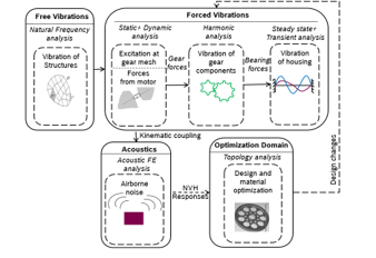Figure 3: Flow of the FE model for dynamic simulations

Damping is the diminution, restriction or prevention of the vibrations. To achieve this, damping elements are introduced to the systems; the addition of these make the power unit more efficient and provide a better ride comfort [23]. When a damped structure, which is initially at rest, is excited with a harmonic load, it has a transient response at first which then fades out quickly. Furthermore, the structure attains a steady state which is characterized by a harmonic response with the same frequency as that of the applied load. The analysis is performed across a frequency sweep by applying the loading at a series of different frequencies and logging its response. This procedure provides solutions to the linear equations of motion when the loading is harmonic. As part of this section, several submodules of the vibro-acoustic template, such as excitations and acoustic influences, are discussed further.

3.2.1. Excitations from the Electric Motor

Electromagnetic (EM) phenomena in drive units can generate undesirable effects such as vibrations. There are, already, a few simulation methods that have been developed for understanding this effect. For instance, paper [29] from Li describes the electromagnetic simulations developed to study the characteristics of flux and EM force under different conditions using FEM, thereby it is utilized to analyze the vibration behavior of the structures. Similarly, paper [30] published by Dupont, focuses on excitations due to electromagnetic phenomena using an electromagnetic FE solver. This excitation is then projected onto the structure mesh of the stator in order to calculate the dynamic response. However, they neglected the effects of excitation due to the transmission errors. Nevertheless, through this work, the radial, tangential and axial forces arising at the stator due to the EM forces are coupled with the mechanical excitations for analyzing the vibration characteristics of the drivetrain.

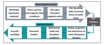Figure 4: Flow for simulating vibration characteristics using EM forces

 Figure 4 describes the flowchart for the calculation of the vibration behavior for the drivetrain based on the EM characteristics. The EM model is prepared using motor geometries and appropriate definitions, such as the phase current. Apart from the calculation of flux and field lines, the simulation also generates an ITEF (Interface for Transfer of Excitation Forces) file. This file consists of information, including RPM, orders and forces at each individual tooth, across discrete time points. The ITEF tool acts as an interface to transfer the forces onto the stator surfaces with radial, tangential and axial components along the frequency spectrum of interest. Later, these forces are used for simulating the harmonics of the drivetrain structures.

3.2.2. Excitations from the Bearings

For further analysis, the gear model with bearings and shafts is simulated. Here, the axial and radial forces at the bearings and other critical areas are calculated. The reaction forces in the simulation are logged in order to retrieve the complete profile of bearing forces. Figure 5 describes the profile of axial forces at the crankshaft after converting into the frequency domain (as an example). The other axes also have analogous profiles with their respective orders and amplitudes. These are not described in detail as the idea was to introduce the user to force amplitude vs. order graphs that are later used in the harmonic excitation step. Information about the simulation model encompassing axial forces and housing structures are explained in the papers [1, 31]. The scale on the y-axis is normalized for non-disclosure purposes.

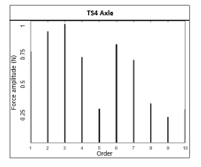Figure 5: Forces at the TS4 axle represented in the frequency domain

3.2.3. Acoustic Mesh

The surface velocities of the housing surfaces create pressure fluctuations of the fluid around them [32]. These disturbances result in noise around the drivetrain. The acoustic pressures and intensities across different distances are estimated with the help of an acoustic FE mesh.

Acoustic elements model the propagation of the acoustic waves and are active only in dynamic analysis procedures. Figure 6 represents the schematic view of the acoustic mesh developed around the drivetrain structure. The terms n_s and n_a indicate the normal vectors of the structural and acoustic mesh, respectively. Furthermore, information corresponding to the coupling between these domains is explained by Sandberg in book [33]. The length of the acoustic elements should be able to capture the maximum frequency of interest. In (10), c, n and h correspond to the speed of sound, number of elements required to capture the wave (generally 5-8) and wavelength, respectively [31].

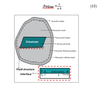Figure 6: Structural, acoustic finite and infinite element model [20]

Exterior surfaces of the structure are tied to the inner surface of the finite acoustic mesh, hence, velocities at the structural surfaces are transferred to the acoustic nodes. Furthermore, the acoustic velocities of nodes can be altered by introducing impedances between the surfaces. Later, the acoustic finite mesh is attached to the acoustic infinite mesh for estimating the pressures at farther distances. The loss effects within the acoustic medium are modeled via volumetric drag and material impedance parameters.

Table 4: Step information for harmonic simulation

Frequency range	300 – 10000 Hz
Applied load	Axial forces (section Excitations from the bearings) and motor forces (section Excitations from the Electric Motor)
Damping factor	0.03 – 0.24 (frequency dependent) (exact values not disclosed)
Step type	Steady state dynamics – modal

3.2.4. Vibration Results

This section provides a brief overview of the acceleration magnitudes for a drive unit simulation. Table 4 indicates the step information such as the frequency range, applied load and damping constants used for calculation of harmonic responses at the housing structure.

Figure 7 describes the surface acceleration recorded at the housing structure element that has the maximum displacement for constant damping factor across the spectrum. The x-axis and y-axis represent the frequency in Hertz and amplitude in Decibels, respectively. Note that these values are scaled appropriately for non-disclosure reasons. The graph shows the influence of the damping ratio on the acceleration magnitude. For lesser damping factors, the peaks tend to be very sharp and for higher damping factors, the amplitudes are reduced and smoothed out. Therefore, the models with damping structures along the transfer path have the potential to create an impedance jump across the intersections, thereby reducing the vibrations. The horizontal line indicate the threshold limit defined using the specification data. The specification sheet including the vibration, sound limits, weight restrictions etc. are obtained from the requirements engineering team, who study the present market situation and analyze the various factors associated with customer satisfaction.

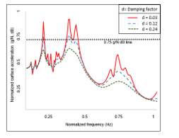Figure 7: Acceleration simulated at a critical node with varying damping factors

Further descriptions of the results are illustrated in section 6, after describing the test setups and connected software.

4. Topology Optimization

Topology optimization starts with an initial model and determines an optimum design by modifying the properties of the material in selected areas, effectively removing elements from the analysis. The numerical methods developed to achieve structural optimization can be classified into two categories: the deterministic method and the probabilistic method. The former uses mathematical programming and a special gradient-based optimizer to perform the optimization. The latter uses heuristic algorithms which are nature-inspired and are developed based on the successful evolutionary behavior of natural systems [34, 35].

For this paper, mostly mathematical programming along with an optimal criteria approach are used in the optimization tasks. The mathematical programming performs iterative changes of the initial design for improving the objective function and fulfilling constraints in each optimization iteration, while the optimal criteria uses mathematical formulations of conditions that characterize the optimum. The design variables are redesigned so that they fulfill the optimal criteria. The main advantages of this method are that it has faster convergence and the speed of this convergence is independent of the number of design variables. Figure 8 shows the flow of data within this optimization module for reducing the stress at critical housing areas.

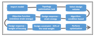Figure 8: Optimization flow for minimizing strain energy

Table 5 describes the variables defined in the Tosca parameter file, which are used in order to optimize the drive unit for the strain energy. A design constraint with 48 % and 27 % of total weight for the housing and cover, respectively, is imposed. The area near the motor, bracket interface, other critical boundaries, etc., must not be changed. Therefore, the model is also given the frozen area for both structures. Minimization of the strain energy of both parts is considered as the objective function of the optimization task. The convergence of results is obtained at optimization iteration number 32. Later, using the Tosca GUI’s Smooth module, visualization of the smoothed, optimized part and the downside of it, i.e., the removed material, is determined.

Table 5: Topology optimization definition for minimizing strain energy

Optimization task	Topology
Objective function	Minimize strain energy / Minimize compliance
Design constraint	Reduction in weight of housing and cover
Strategy	Topology sensitivity
Iteration stop	50

Figure 9 describes the reduction in strain energy through the optimization simulation. The smoothed results from the Tosca are revised in the CAD software and finally new housing and cover parts with 55 % and 31 % of the original parts are obtained.

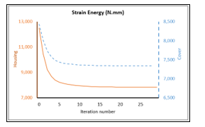Figure 9: Strain energy vs. optimization iteration

Once the optimization task has been accomplished, new components with a mixture of the two materials can be defined. It is understood that the existing structures, i.e., the resulting elements of the optimization, have the maximum stress and strain energy, therefore, these elements were retained during the optimization. These structures are referred to as skeletons in the further sections of the work. This mechanical optimization shows that it is possible to simplify the geometry of the housing and cover whilst maintaining the stiffness of the structure. The metal skeleton can then be provided with a plastic insert in order to close and seal the drive unit.

In the next step, removed elements (negative volume) are replaced with different plastic materials to obtain the weight reduction in comparison with the original parts and, at the same time, curtail the stress limits below the thresholds.

Table 6: Maximum stress, drivetrain weight and percentage mass in comparison with original drive unit

Material	Max stress (MPa)	Drivetrain weight (gm)	Optimized drivetrain mass in %
Mg Skeleton	1530	243	47
EP43	380.6	425	82
Akulon	581.2	425	82
Delrin	361.9	467	90
Polyfort	553.4	396	76

The results in Table 6 show that the addition of plastic significantly reduces the stresses in the parts compared to the pure metal skeleton. Only a few areas of the housing have stresses that exceed the yield limit. In addition, these areas are thin and very localized. The geometry of these zones must be revised in CAD software in order to bring their maximum stress below the fracture limit.

Among the various plastics used, Delrin offers the lowest maximum stress at 361.9 MPa, while the addition of Polyfort enables the best weight savings. In fact, the magnesium skeleton supplemented with Polyfort accounts for 76 % of the mass of the original DU. EP43 is a compromise between these two cases and represents the best optimization solution. Indeed, when added to the magnesium skeleton, this allows a maximum tension of 380.6 MPa to be obtained, whilst the end part (skeleton and plastic) comprises 82 % of the original drivetrain mass. This weight saving of almost 20 % represents a potential improvement in the drivetrain. The geometry of this new structure must be revised for it to be constructed. In addition, thermal aspects must also be considered. Indeed, the structure must allow the thermal dissipation of the heat generated by the engine and transmission during the operation of the DU. The connection between metal and plastic must adapt to the different thermal expansions of the materials to ensure a perfect seal during operation.

5. Dynamic Optimization

Developing a sensible combination of objective functions and constraints is one of the most challenging steps in applying topology optimization. For the design of dynamic systems, structural vibration control is the most essential consideration. The objective of this type of optimization is to achieve the optimal material layout for the load-bearing components.

Figure 10 describes the flow of the optimization module to optimize the structural dynamics of the housing and cover, thereby improving the drivetrain. The two basic parts (cover and housing) are covered with an envelope volume (design volume). The internal forces, the electromagnetic forces of the motor and the transmission from section 3.2 are applied. The displacements of frame interface points are measured, which enables reaction forces to be calculated. The aim of the dynamic optimization is then to minimize the amplitude of the reaction forces in order to reduce the noise generated by the drive unit during its operation. For this purpose, the optimization software removes material from the design volume to form the optimal ribs. The complete design volume (from both housing and cover) weighed 1.25 kg at the beginning of the simulation. The restriction introduced via the volume constraint corresponds to a final weight corresponding to 30 % of the initial weight. This optimization is carried out in 42 iterations over 38 hours to give a final weight of 312 gm (i.e., approximately 26 % of its starting weight).

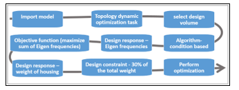Figure 10: Optimization flow for linear dynamics

Table 7 illustrates the variables defined in the Tosca parameter file that tries to optimize the drive unit for the dynamic characteristics.

Table 7: Topology optimization definition for reducing the noise level

Optimization task	Topology
Objective function	Minimize the vibration and sound levels
Design constraint	Reduction in weight and stress of housing and cover
Strategy	Topology sensitivity
Iteration stop	80

The Frequency Response Function (FRF) is a frequency-based function used to identify the resonant frequencies, damping and mode shapes of the structure. This expresses the frequency domain relationship between an input (force) and output (acceleration) of a linear, time-invariant system. Figure 11 describes a FRF graph for the mean acceleration measured at the critical interface points. This optimization shows a decrease in the maximum acceleration by 4.2 dB. This reduction is greater at higher frequencies and reaches 12 dB compared to the initial drive unit. Overall, the acceleration of the optimized model lies well within the thresholds (limits shown in Figure 11).

Similarly, Figure 12 represents the octave spectrum simulated at 1000 mm distance from the main housing structure. This figure compares the sound pressure levels of the optimized and original drivetrain structures. Optimization shows a decrease in the sound pressure level by 6.2 dB at the frequency spectrum band with the maximum amplitude. This difference is greater at higher frequencies and reaches 13.4 dB compared to the original drivetrain. Overall, the acoustic values of the optimized model lie well within the thresholds.

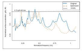Figure 11: Vibration plot of optimized vs. original drivetrain structure

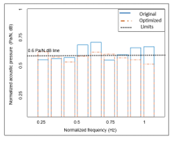Figure 12: Octave (acoustic) plot of optimized vs. original drivetrain structure

6. Method Verification

This part of the paper describes the validation of the methodology generated using the simulation techniques in section 3.2. Initially, the experimental setup developed for a DU variant is illustrated. Later, the FE model verification is shown using the values of surface acceleration and acoustic pressure.

6.1. Experimental Setup

Experiments are performed to verify the surrounding pressure and surface velocities of the current drivetrain variant obtained from the numerical calculations. Figure 13 illustrates the schematic experimental setup of the drivetrain and corresponding measuring devices. The absorber box is used to isolate the powertrain vibrations from the surroundings. The different forms of the dashed lines indicate the surface velocities and acoustic fluctuations respectively.

RPM and motor torque profiles are considered as inputs for simulations and experimental runs. The Polytec laser vibrometer is used for the measurement of exterior vibrations of the housing and cover surfaces [36]. Acceleration sensors are mounted to obtain accelerations at precise locations. The sound pressure level is measured using the acoustic camera (from Head Acoustics) and microphones installed at a distance of 1000 mm [37]. LMS software serves as a central node to send the force reference signals and also to record the vibrations and noise [38]. Finally, after the analysis of multiple DU variants for various torque and RPM profiles, the Campbell and spectral plots are generated.

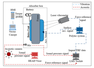Figure 13: Experimental model for measuring noise and vibration [1]

6.2. Numerical Validation

This section attempts to establish the relationship between the experimental results and the FE values. As a part of it, the first step is to validate the model components for their natural frequencies. It aids in verifying properties like damping factors, Eigen forms and frequencies of the components (not shown in this paper). The comparison of Eigen forms between the Experiment Modal Analysis (EMA) and FE frequency analysis helped to determine the variables like loss coefficients for the spectrum of interest. This data is further used for simulating the harmonic step using the steady state dynamic solution technique. Validating the complete drivetrain at the first go can be extremely hard due to complexities associated in the system. At the start, individual structures are verified and later for the combined structures. Validating various combination of structures enabled for studying the properties of damping associated with contact.

The presence of permanent deformations can alter the dynamic characteristics. Hence, before performing the harmonic analysis of complete drivetrain, the structures are checked for plastic deformations for the static load case. In the end, the damping and material values obtained from the combined structures are used for the simulation and validation of the forced excitation (Figure 14) of the complete drivetrain. Here, an excitation with a torque (2.5 N.m), RPM (0-2500) and appropriate boundaries are used.

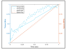Figure 14: Torque and RPM profiles vs. time

Figure 15 shows the FRF plot of the simulation and experimental results for the vibrations of a DU variant (using the template discussed in section 3.2). The x-axis corresponds to the frequency spectrum. The y-axis represents the surface velocity of a critical node on the exterior surface of the drivetrain (g/N, dB). The numbers shown on the graph correspond to the resonance frequencies. These peaks indicate the presence of Eigen frequencies for the drivetrain components. Figure 16 describes the octave plot (1/3rd) of the acoustic quantity. The y-axis of Figure 16 represents the acoustic pressures (Pa/N, dB). The simulation and experimental values shown in Figure 15 and Figure 16 have a deviation of around 8.78 % and 4.38 % (on average), respectively.

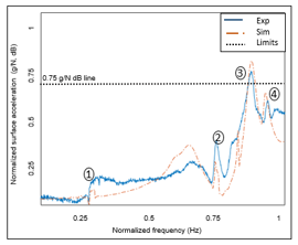Figure 15: FRF vibration plot – Experimental vs. Simulated

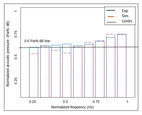Figure 16: Sound octave spectrum – Experimental vs. Simulated

7. Conclusion

A numerical modeling method for the drivetrain with the aim of understanding the structural properties, such as stress, strain energy, compliance, surface velocities and acoustic pressure is proposed. First, a static model template with its appropriate forces and boundaries is shown. The model is then simulated for the worst load case, i.e., the uphill condition. The vibro-acoustic template introduces the user to topics related to electromagnetic influences, axial forces and structural fluid coupling. Furthermore, the harmonic forces emanating from the bearings and the motor are included into the template. Harmonic analysis is used to calculate the surface acceleration at the housings and the sound pressure in the surroundings. The next section describes two different optimized models with targets of minimizing strain energy and surface velocities. These two tasks cannot be encompassed into one single model as the solver for both the cases is different. The first scenario dealt with a static non-linear model and the second focused on the structural dynamic characteristics. The validations are illustrated by comparing the frequency curves of simulations and experiments.

The dynamic responses described in this paper are considerably improved in comparison with the multi-body models that are illustrated in the state of the art [1]. Although the results from physical modeling approach [1] are promising, it failed in providing the information like the locations with higher vibration amplitudes in the structures. The FE method helped to realize the critical areas of the structures and to develop high-level models for calculating the acoustic reactions at precise distances. The other prior art approaches such as [6, 8, 9, 17] dealt with a single facet of the problem such as the analysis of the transmission vibrations or just a static optimization or FE modeling etc., for the traditional drive trains. The approach described in this paper aided in building a complete flow analyzing the excitations from several sources on the gears, the motor, the bearings and the housing structures for the electromechanical drives. The method also helped in connecting the static and dynamic domain to build a model with minimized deformations and vibrations simultaneously (Figure 3).

Although the simulation results obtained do not fully complement with the experiments, a substantial 78 % of results are decently fitted. The deviations between results are caused by reasons such as device calibrations, simulation errors and complexities in representing the physical significance of drivetrain parts. Improvements such as better contact, acoustic modeling in simulations and more robust test setups like anechoic chambers can aid in mitigating these differences. At the fluid structure boundary, the simulation setups transfer all the velocities from structural to acoustic domain, while in reality there is energy dissipation due to experimental conditions. Although the losses can be included using impedance boundaries in the FE, a detailed study needs to be performed to define the exact admittance and volumetric drag coefficients. Overall, the system method developed appears to have the potential to predict the NVH characteristics and can be considered for analyzing the optimized drivetrain models.

8. Outlook

Since the FE values obtained for the original drivetrain model are close enough to the experimental results, the next major step would be to build the real parts of the optimized housing and cover. It would be essential to perform validation on the improvised designs obtained from Tosca.

Other aspects such as thermal fluctuations inside drivetrain can also influence the stresses and linear dynamic characteristics of the structures. The developed simulation templates can thus be further integrated into other areas such as the thermal, control systems and the electrical system model, via heterogeneous modeling techniques.

Also, wear among the gears could affect the noise of the drive train. For example, the methods described in paper [39] can be used as a basis for understanding the dependence of the abrasion mechanism on the noise emission of the drivetrain.

Conflict of Interest

The authors declare no conflict of interest.

1. Y. Kolluru, R. Doelling, L. Hedrich, Numerical simulations of vibro acoustic behaviors related to drive train assemblies, in 2019 International Symposium on Systems Engineering (ISSE), 2019. https://doi.org/10.1109/ISSE46696.2019.8984458
2. T. Kato, R. Mizutani, H. Matsumoto, K. Yamamoto, Advanced technologies of traction motor for automobile, in 2013 IEEE ECCE Asia Downunder, IEEE, 147–152, 2013. https://doi.org/10.1109/ECCE-Asia.2013.6579088
3. J. de Santiago, H. Bernho_, B. Ekergard, S. Eriksson, S. Ferhatovic, R. Waters, M. Leijon, Electrical motor drivelines in commercial all-electric vehicles: A review, IEEE Transactions on Vehicular Technology – IEEE TRANS VEH TECHNOL, 61, 475–484, 2012. https://doi.org/10.1109/TVT.2011.2177873
4. E. Rask, M. Duoba, H. Lohse-Busch, Recent hybrid electric vehicle trends and technologies, in 2011 IEEE Vehicle Power and Propulsion Conference, IEEE, 1–6, 2011. https://doi.org/ 10.1109/VPPC.2011.6043172
5. J. M. Rodriguez, R. Meneses, J. Orus, Active vibration control for electric vehicle compliant drivetrains, in IECON 2013-39th Annual Conference of the IEEE Industrial Electronics Society, IEEE, 2590–2595, 2013. https://doi.org/ 10.1109/IECON.2013.6699539
6. Y. Ito, S. Tomura, K. Moriya, Vibration-reducing motor control for hybrid vehicles, RD Review of Toyota CRDL, 37–43, 2005. https://www.tytlabs.com/english/review/rev402epdf/e402_037ito.pdf, last accessed 2020/21/07
7.  K. Jensen, Optimising stress constrained structural optimisation, in 23rd International Meshing Roundtable (IMR), Elsevier, 2014. https://imr.sandia.gov/papers/abstracts/Je751.html, last accessed 2020/21/07
8. E. Hinton, J. Sienz, Fully stressed topological design of structures using an evolutionary procedure, Engineering Computations: Int J for Computer-Aided Engineering 12, 229–244, 1993. https://doi.org/10.1108/02644409510799578
9.  H. Eschenauer, A. Schumacher, T. Vietor, Decision makings for initial designs made of advanced materials, in Topology design of structures, Springer, 469–480, 1993. https://doi.org/10.1007/978-94-011-1804-0_33
10.  Y. M. Xie, G. P. Steven, A simple evolutionary procedure for structural optimization, Computers & structures 49, 885–896, 1993. https://doi.org/10.1016/0045-7949(93)90035-C
11. K. Suzuki, N. Kikuchi, Layout optimization using the homogenization method, in Optimization of large structural systems, Springer, 157–175, 1993. https://doi.org/10.1007/978-94-010-9577-8_7
12. K. Mao, An approach for powertrain gear transmission error prediction using the non-linear finite element method, Proceedings of the Institution of Mechanical Engineers, Part D: Journal of Automobile Engineering 220, 1455–1463, 2006. https://doi.org/10.1243/09544070JAUTO251
13. Y.-C. Chen, C.-B. Tsay, Stress analysis of a helical gear set with localized bearing contact, Finite Elements in Analysis and Design 38, 707–723, 2008. https://doi.org/10.1016/S0168-874X(01)00100-7
14. D. A. Crolla, D. Cao, The impact of hybrid and electric powertrains on vehicle dynamics, control systems and energy regeneration, Vehicle system dynamics 50, 95–109, 2012. https://doi.org/10.1080/00423114.2012.676651
15. R. Anderl, Simulations with NX: Kinematics, FEM, CFD, EM and Data Management. with Numerous Examples of NX 9, Hanser eLibrary, Hanser Publications, 2014.
16. S. Iyengar, R. N. Elements of Mechanical Vibration. India, I.K. International Publishing House Pvt. Limited, 2010.
17. J. A. Morgan, M. R. Dhulipudi, R. Y. Yakoub, A. D. Lewis, Gear mesh excitation models for assessing gear rattle and gear whine of torque transmission systems with planetary gear sets, SAE Transactions, 1780–1789, 2007. https://doi.org/10.4271/2007-01-2245
18. H. Allik, Accuracy of infinite elements in structural acoustics modeling, The Journal of the Acoustical Society of America 77, 1985. https://doi.org/10.1121/1.2022426
19. R.G. Grimes, J. G. Lewis, and H. D. Simon, A Shifted Block Lanczos Algorithm for Solving Sparse Symmetric Generalized Eigenproblems, SIAM Journal on Matrix Analysis and Application, 228–272, 1994. https://doi.org/10.1137/S0895479888151111
20. R. C. Shieh, Massively parallel structural design using stochastic optimization and mixed neural net/finite element analysis methods, Computing Systems in Engineering 5, 455–467, 1994. https://doi.org/10.1016/0956-0521(94)90026-4
21. M. P. Bendsoe, N. Kikuchi, Generating optimal topologies in structural design using a homogenization method, Computer Methods in Applied Mechanics and Engineering, 197-224, 1988. https://doi.org/10.1016/0045-7825(88)90086-2
22. W. Desmet and D. Vandepitte, Numerical Acoustics: Finite Element Modeling for Acoustics, ISAAC 13- International Seminar on Applied Acoustics, 37-85, 2005.
23. Y. Kolluru, R. Doelling, L. Hedrich, Multi domain modeling of NVH for electro-mechanical drives – accepted for publication, in 2020 Integrating Seamlessly NVH, 2020. https://saemobilus.sae.org/content/2020-01-1584, last accessed 2020/21/07
24. M.P. Bendsoe and O. Sigmund, Topology optimization: Theory, methods and applications, Springer-Verlag, Berlin Heidelberg, 2003.
25. K. Svanberg, The method of moving asymptotes – A new method for structural optimization. International Journal for Numerical Methods in Engineering, 359-373, 1987. https://doi.org/10.1002/nme.1620240207
26. Simulia, Simulia User Assistance Guide 2018, About Abaqus and Tosca, Dassault Systems Simulia Corp, 2018. http://si0vm1337.de.bosch.com:8081/EstProdDocs2018/English/DSSIMULIA_Established.htm?show=SIMULIA_Established_FrontmatterMap/DSDocAbaqus.htm, last accessed 2020/21/07
27. I. 4210-8:2014, Cycles – safety requirements for bicycles – part 8: Pedal and drive system test methods (iso 4210- 8:2014), Online Browsing Platform 1, 2014. https://www.iso.org/standard/59915.html, last accessed 2020/21/07
28. P. Wriggers, Contact mechanics, Prentice Hall, New Jersey, 2007.
29. R. Li, X. Peng, W. Wei, Electromagnetic vibration simulation of a 250 mw large hydropower generator with rotor eccentricity and rotor deformation, Energies 10, 2017. https://doi.org/10.3390/en10122155
30. J.-B. Dupont, P. Bouvet, Multiphysics modelling to simulate the noise of an automotive electric motor, in 2012 Integrating Seamlessly NVH, 2012. https://doi.org/10.4271/2012-01-1520
31. Y. Kolluru, R. Doelling, L. Hedrich, Numerical Analysis of the Influences of Wear on the Vibrations of Power Units – accepted for publication, in 2020 Integrating Seamlessly NVH, 1–12, 2020. https://saemobilus.sae.org/content/2020-01-1506, last accessed 2020/21/07
32. L. Kinsler, Fundamentals of Acoustics, John Wiley & Sons Australia, Limited, 2000.
33. G. Sandberg, R. Ohayon, Computational Aspects of Structural Acoustics and Vibration, CISM International Centre for Mechanical Sciences, Springer Vienna, 2009.
34. R. Picelli, S. Townsend, C. Brampton, J. Norato, H. Kim, Stress based shape and topology optimization with the level set method, Computer Methods in Applied Mechanics and Engineering 329, 1-23, 2018. https://doi.org/10.1016/j.cma.2017.09.001
35. C. Mitropoulou, Y. Fourkiotis, N. Lagaros, M. Karlaftis, Evolution Strategies Based Metaheuristics in Structural Design Optimization, 79–102, 2013. https://doi.org/B978-0-12-398364-0.00004-8
36. P. G. Technology, Vibrometer measurements methods, 2019. https://www.polytec.com/eu/vibrometry/technology/, last accessed 2020/21/07
37. H. acoustics, Acoustic camera / head visor(code /5000_) handbook., 2016. https://www.head-acoustics.com/eng/nvh_head-visor.htm, last accessed 2020/21/07
38. Siemens, Lms test.lab, Analysis and structural design manual, Siemens Industry Software, 2015. http://citeseerx.ist.psu.edu/viewdoc/download?doi=10.1.1.372.6925&rep=rep1&type=pdf, last accessed 2020/21/07
39. Y.Kolluru, R.Doelling, L. Hedrich, Wear estimation using FEM and machine learning techniques, in 2019 ECOTRIB conference, 176–178, 2019. https://ecotrib2019.oetg.at/program2.

(Click Here)

(Click Here)