1. Introduction

Man’s dream of flying has been fulfilled by hot air balloons by the end of the 18^th century and the realisation of a controlled flight was done by the design proposal of Jean-Baptiste Meusnier. Airship technology has a great history starting from the hot air balloons used in the medieval ages and has been widely used in the 19^th century. Unfortunately, the interest in airships has been lost due to the high maintenance cost, drastic developments in air crafts and helicopters and some catastrophic tragedies such as the Hindenburg disaster [1]. By the end of the 20^th century, a resurgence in the interest in airships by researchers and military agencies has occurred (as shown in Figure 1) due to the low speed, long endurance, economic, noiseless and eco-friendly operation of airships. Major applications [2] of airships include transportation of war equipment, intelligence, surveillance, reconnaissance, advertisement, telecommunication, monitoring and inspection of climate and environmental effects, inspection of man-made structures such as buildings, pipelines, railway network, and power lines, planning for urban development, research, exploration and so on.

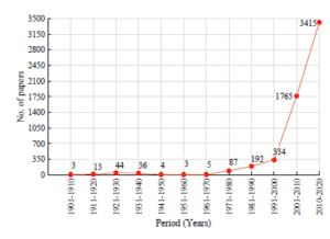
Figure 1: Number of papers published in the field of LTA vehicles (Source: Scopus database)

The airship based application has to be modelled to reflect the expected behaviour. Like any other complex system, dynamic modelling of an airship is one of the challenging areas for researchers in this field. Dynamic modelling of Lighter-Than-Air (LTA) vehicles differ from other members of aerial vehicles such as helicopters and air crafts. There is a close similarity between the dynamics of an airship and an underwater vehicle [3], which researchers exploited for modelling the airship in the early stage of research [4]. A detailed survey of the dynamic modelling of the airship is presented in [1] along with the details of wind tunnel tests; which are being utilized by researchers for the dynamic modelling and structural design of airships. A system level mathematical modelling of a high altitude airship is presented in [5]. The presented model includes the airship dynamic model, solar power system model and atmosphere models. The aerodynamic modeling of the airship was done using the geometrical data available from the literature. A linearized longitudinal and lateral dynamic models of an airship is presented in [6]. An analysis of different stability modes for the two linear models was presented. A dynamic model is presented for an airship in [7] which utilizes the geometrical aerodynamic parameters for the model. A simulation methodology is also presented to demonstrate the effectiveness of the developed model using MATLAB ^R .

Most of the above cited works on the dynamic modelling of airships have utilised the available database or the method of practical extraction from the actual system for obtaining the model parameters such as the aerodynamic coefficients. There are various methods by which we can estimate the parameters included in the aerodynamic model such as CFD based methods [8], experimental methods using wind tunnel [4, 9] and analytical methods [10]. Computational Fluid Dynamics (CFD) tools can be used to extract the aerodynamic coefficients for airship geometries [11, 12]. A method of extracting the force and moment coefficients of an airship using CFD and Fourier analysis is presented in [11]. Forced sinusoidal oscillations are used in the longitudinal direction to extract the force and moment coefficients. A specialised computational tool used for the aerodynamic coefficient extraction is presented in [12]. The major drawbacks of CFD based analysis are the inability to model the geometry accurately, computational cost and time taken for simulation. The traditional way is to use wind tunnel testing for the extraction of aerodynamic coefficients [4, 9]. An analytical method for calculating the aerodynamic coefficients and other control derivatives is presented in [9]. The method is heavily dependent on the wind tunnel test results. A detailed investigation of LOTTE airship using wind tunnel is presented in [4] in which the force and moment coefficients, pressure distributions and the flow visualization were elaborately discussed. There are practical difficulties in this method such as the size limitation of the test section of the wind tunnel, difficulties in the installation and inaccurate measurements, inaccuracies due to the blockages in the tunnel, etc. Most accurate and realistic data for the calculation of those coefficients can be obtained through actual test flights [10]. But it is not always feasible to conduct flight tests because of fuel consumption, unsteady atmosphere conditions, etc. There are a lot of works carried out in this context which are trying to reduce the efforts in the calculation. A method which requires no experimental data for calculating the aerodynamic coefficients using geometrical parameters is presented in [13]. The problem with this method is the inability to generalise the method to all class of airships. The parameters specified in the study are particularly available for a certain class of airships only. The digital DATCOM software based on Fortran is reported to be useful in the calculation of the aerodynamic coefficients. Such a work is presented in [14, 15] which used the DATCOM to predict the aerodynamic coefficients for a high altitude airship to manoeuvre at an altitude of 21000 m. This method is also limited to the available datasets in the DATCOM database.

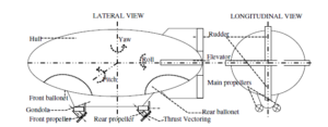
Figure 2: Basic components, actuators, and degrees of freedom of a double ellipsoid airship [16]

There is no doubt that the above cited works are providing enough light to the field of aerodynamic modelling of airships. As per the difficulties posed by those methods, it is evident that there is still scope for research in this field using methods which need not rely much on experimental data, complex geometry development for CFD, etc. The aim of this work is to present a study on the aerodynamic modelling of a high altitude airship. The current study is motivated by the work presented in [13] which describes a method of aerodynamic modeling for the aircraft with a little experimental data. We are investigating the same technique for a high altitude airship which is modelled using a modified set of aircraft equations of motion. The main advantage of this method is that the experimental data required for the modelling is considerably less. The remaining paper is presented in five sections. After the introduction and literature survey presented in Section 1, a brief description of the principle of operation of airships is given in Section 2 as a preliminary note. Different components of the airship, application of each component, principle of lift and hovering are also presented in Section 2. Section 3 discusses the complete dynamic modelling of a high altitude airship with a detailed study on aerodynamic modelling. Section 4 discusses the simulation results and their analysis. Simulation of the aerodynamic coefficients for different flight conditions and an open loop simulation of the airship are presented along with the results. Finally the conclusions and future works are presented in Section 5.

2. Airship Principle of Operation

The basic principle behind the operation of airships is the natural buoyancy of LTA gases such as hot air, helium and hydrogen. The concept of airship came from the basic hot air balloon, which uses the buoyancy property for lift generation. But to use it as a vehicle, there should be some modifications made on the balloon such as the streamlined body to reduce the air resistance and to enhance the aerodynamic properties. Figure 2 shows the major parts of a double ellipsoid airship [16]. The main body, which is known as the hull, occupies the large volume of LTA gas. Based on its structure, airships are classified as non-rigid, semi rigid and rigid airships. Non-rigid airships, also known as blimps, do not have any rigid structure to maintain its streamlined shape. It is maintained by the pressure inside the envelope. While rigid and semi rigid airships have a fully supported or partial mechanical structure on which the hull envelope is attached. Hull houses the pressure controlling ballonets, which can even control the altitude and pitch of airships. The pressure and thereby volume of the LTA gas may vary with altitude, which results in the expansion and contraction of the gas accordingly. As altitude increases, the helium expands which pushes the air in ballonets out. This will continue till the pressure height which is the designed maximum altitude of operation. Beyond the pressure height, the safety valve will release helium to avoid bursting.

Thrusters or propellers are the aerostatic actuators used for longitudinal and lateral movement of airships. A pair of propellers are placed on both sides of the gondola which provides the forward thrust. Thrust vectoring can be included to have a longitudinal freedom when the aerodynamic actuators are not active due to low wind. Apart from these main propellers, stern propellers may be used for providing a lateral degree of freedom when the aerodynamic surfaces cannot provide much actuation. Aerodynamic control surfaces are provided at the stern end of airships which can control the yaw, roll, and pitch degrees of motion. These control surfaces can be either designed as a ‘+’ configuration or ‘X’ configuration. Elevators produce a pitch degree when they act together in the same direction and a roll degree can be generated by differentially actuating the elevators. Yaw is provided by rudders which are the vertical control surfaces. Another part of the airship is the ballast mechanism to control the pitch. By using solid or liquid as a movable mass, the pitch can be controlled by manipulating the location of the centre of gravity of the airship, and sometimes the gondola completely can be the ballast.

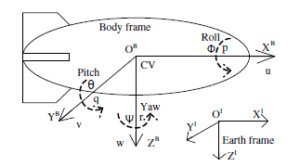
Figure 3: The reference frames used for the dynamic model along with the linear and angular position and velocities [16]

The airship considered in this study is a high altitude airship which is intended to operate at 21000m. The hull is of Gertler shape with four tail fins (as shown in Figure 2) and two thrusters. There are some assumptions based on which the following analysis is carried out. They are,

• Hull volume is constant throughout the simulation
• Structure of the airship is rigid
• The airship geometry is symmetric in the XZ plane
• Airship is at neutral buoyant condition
• A flat earth approximation is followed

3. Dynamic Model

As mentioned in Section 1, the dynamic modelling of an airship differs largely from that of an aircraft. The displaced Centre of Gravity (CoG) from the Centre of Volume (CoV) and the effect of the added mass of the surrounding air are the main contrasting features of LTA vehicle models. The displacement of the CoG vertically downwards of the CoV is to provide unconditional stability for the airship. The tendency of rotation will be counteracted by the downward displaced CoG. Even though the mathematical model of an airship differs from that of an aircraft model, it is possible to include the added mass, buoyancy and the aerodynamic properties of the airship to the aircraft model. The advantages of this methodology are the availability of well-established flight dynamic equations, availability of experimental data for different flight and airship configurations and more insight into the dynamic behaviour of the airship in the light of aircraft dynamics.

3.1        A mathematical model for an airship

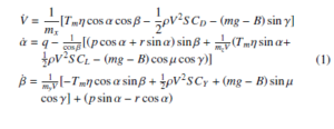
For deriving the dynamic equations of a rigid body there should be a coordinate system which can properly behold the complexity, degrees of freedom and application requirements. There are mainly three reference frames earth fixed inertial frame, wind frame and body frame. The position and orientation of an object in the atmosphere with respect to the earth can be obtained with the help of earth fixed inertial reference frame. In the same way, the forces and moments of a moving body are not only depending on the velocity with respect to earth but also to the surrounding air itself. This leads to the consideration of an atmosphere fixed reference frame i.e., wind reference frame which is a moving frame with respect to earth but not with respect to the vehicle. Another set of a reference frame is the body fixed frame which is fixed to the CoV and is moving with the vehicle. The earth fixed inertia and the body fixed reference frame are shown in Figure 3 (wind frame is not included since it is considered temporarily during the derivation). The inertia frame O_IX_IY_IZ_I is having the orientation as X_I pointing towards the north, Y_I towards the east and Z_I towards the centre of the earth. Similarly, the body frame O_BX_BY_BZ_B has its centre at the CoV of the airship and X_B pointing towards the nose of the vehicle, Y_B towards the right side wing and Z_B pointing downwards perpendicular to X_B and Y_B. The wind frame is used only during the derivation of equations and the final equations will be expressed in terms of the earth and body frames only. In a general way, the dynamic equations for an airship can be represented as follows,

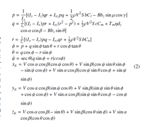
where

sinγ = cosαcosβsinθ − sinβsinφcosθ − sinαcosβ cosφcosθ

sinµcosγ = cosαsinβsinθ + cosβsinφcosθ − sinα sinβcosφcosθ

cosµcosγ = sinθ sinα + cosαcosφcosθ

where the states [V α β p q r φ θ ψ x_E y_E z_E]^T are the forward velocity, angle of attack, side slip angle, body axis role, pitch and yaw rates, roll, pitch and yaw angles and position coordinate in the earth frame respectively, m_x,m_y and m_z are the components of apparent mass, T_m is the maximum engine thrust, η is the throttle ratio, ρ is the density, S is the wing planform area, c is the chord, b is the wingspan, b_z is the point of action of buoyant force along the Z_B direction, d_z is the point of action of thrust along the Z_B direction, B is the buoyant force, m is the airship mass, I_x, I_y, I_z, I_xz are the inertia components, C_D,C_L,C_Y are the drag, lift and side force coefficients, C_l,C_m,C_n are the rolling, yawing and pitching moment coefficients.

3.2        Aerodynamic coefficients

The set of equations described in Section 3.1 are modified aircraft equations to demonstrate the dynamics of a high altitude airship. The aerodynamic parameters in the equation such as

C_D,C_L,C_Y,C_l,C_m and C_n are the major design parameters of the airship. There is an analytical method for the calculation of the aerodynamic coefficients for aircraft using the actuator values [13].

Since the airship model used in this paper is modified from the same aircraft model, this method is investigating for the airship in this paper. The method calculates the aerodynamic coefficients as a function of α, β, p, q, r, δ_e, δ_a and δ_r. The set of equations for the calculation of aerodynamic coefficients are given by equations (3) to (8).

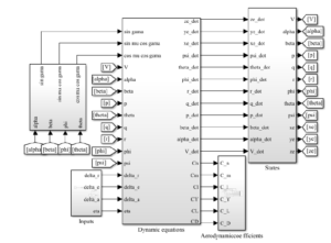
Figure 4: Simulink block diagram of the simulation of airship

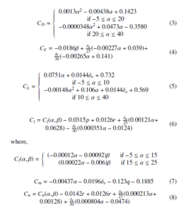
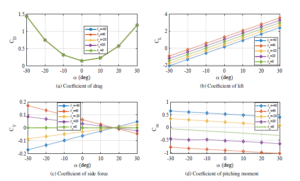
Figure 6: Simulation results of the aerodynamic coefficients given by (3)-(8) for various values of δ_e

where δ_e,δ_a and δ_r are the deflection of the elevator, aileron and rudder respectively.

4. Results and Discussion

4.1        Simulation

The model of the airship is implemented using MATLAB ^R Simulink 2018a. Simulink block diagram of the simulation is as shown in Figure 4. The ‘Dynamic equations’ block shown in Figure 4 holds the realisation of airship dynamic equations given in (1) and (2). The ‘Aerodynamic coefficients’ block in Figure 4 consists of the realisation of coefficients given in (3) – (8). As a representative figure, the simulink block diagram of the coefficient of drag expressed in (3) is shown in Figure 5. The parameters used for the simulation are given in Table 1. ODE45 solver with variable time step execution is used for the simulation. Five sets of elevator deflection angles are used for the simulation.

4.2        Simulation results

The method of obtaining aerodynamic coefficients explained in (3) (8) is directly applicable to aircraft. It can be extended to airships also. Since there is no aileron for the airship, the value of δ_a is taken as same as δ_e. The aerodynamic coefficients represented using equations (3)-(8) are obtained for different values of α and δ_e are shown in Figure 6. C_D, C_L, C_Y and C_m are shown in Figure 6 and C_l and C_n are not shown since their values are zero for the simulated conditions. Even though we have shown the coefficients for a wide range of angle of attack starting from −30 to 30 degrees, the airship simulation later in this section shows that the angle of attack remains within 10 degrees. It is evident that the angle of attack obtained in our simulation is far below the stall angle for a stream lined airship [17]. So the problem of stalling is not in the scope of this work.

Table 1: Model parameters used for the simulation

No.	Parameter	Value	Unit
1	m	23145	kg
2	Ix	17400000	kgm2
3	Iy	245264282	kgm2
4	Iz	245264282	kgm2
5	Ixz	1920000	kgm2
6	Tm	6000	N
7	η	23145	kg
8	mx	25032	kg
9	my	43044	kg
10	mz	43044	kg
11	Tm	6000	N
12	ρ	0.0767	kgm3
13	S	4748	m2
14	bz	16.43	m
15	dz	14.67	m
16	c	68.9	m
17	b	68.9	m

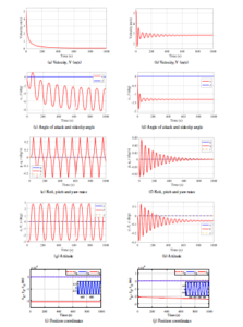
Figure 7: Simulation results for the airship model for zero thrust shown in the first column((a), (c), (e), (g), (i) and 0.1836 throttle ratio shown in the second column ((b), (d), (f), (h), (j))

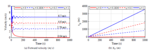
Figure 8: Simulation results of the forward velocity and position along x axis for different η values

Coefficient of drag, C_D is given in Figure 6 (a). The higher values of drag at the higher angle of attacks are as expected and it is clear from the results that there is no effect of δ_e on the drag coefficient of the airship. Even though the coefficients are given for a wide range of angle of attacks, the normal operation (except the take off and landing) of airships will be in a small angle of attack.

The drag coefficient at zero angle of attack is 0.1432.

Coefficient of lift, C_L, seems to have a wide range of deviation for the simulated angle of attacks as shown in Figure 6 (b). The model shows a positive lift at zero angle of attack and the above, which is a characteristic peculiarity of airships. Coefficient of side force, C_Y, and the coefficient of pitching moment, C_m are shown in Figure 6 (c) and (d) respectively.

These extracted aerodynamic coefficients are used for the model given in (1) and (2) and are simulated to see the response for different inputs. Some of them are given in the following paragraphs.

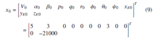
The initial condition for the 9 state variables used in (1) and (2) is as given as follows;

A zero input simulation of the airship is shown in the first column of Figure 7. The simulation was run for 1000 seconds. The velocity of the airship is asymptotically settling to zero as shown in Figure 7 (a). There is an oscillating negative angle of attack around −7 degree which causes a slight decrease in the altitude of the airship from the initial altitude. The side slip angle remains zero throughout the simulation as shown in Figure 7 (c). Figure 7 (e) shows the roll, pitch and yaw rates of the airship. The roll and yaw rates remained at zero throughout the simulation, but the pitch rate shows an oscillation as shown in Figure 7 (e). These oscillations are reflected in the attitude of the airship also. Figure 7 (g) shows the oscillatory pitch angle and the zero roll and yaw angles. The position of the airship with respect to the inertial frame are shown in Figure 7 (i). It is clear from the figure that the airship is staying at the initial position through out the simulation. There are slight deviations in the y direction but it is negligibly small. There is a slight oscillation in the y_E of the order of 1 m/s which is shown in Figure 7 (i).

Another set of results are shown in the second column of Figure 7 with a minimum throttle ratio of 0.1836 by keeping all other inputs zero. The velocity is settling at 2.8 m/s after a prominent overshoot and oscillations as shown in Figure 7 (b). The angle of attack and side slip angle are shown in Figure 7 (d). There is a large improvement in the magnitude of the negative angle of attack. Now the angle is −1.3 degree which can be expected due to the thrust generation off to the centre of gravity. The side slip angle remains zero. The pitch rate oscillation dies out asymptotically as shown in Figure 7 (f). The roll and yaw rates are remaining the same as in the first

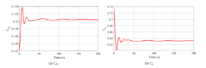
Figure 9: Transient response of the coefficient of drag and lift

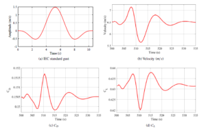
Figure 10: Gust response of the velocity, coefficient of drag and lift

case. The attitude of the airship is shown in Figure 7 (h) in which the pitch angle θ has a negative angle of −0.6 degree. This indicates the inherent dynamics of the airship due to the displaced CoG from the CoV. An active elevator control is necessary to overcome this. Otherwise, the station keeping of the airship at the desired altitude will be difficult. The roll and yaw angles remain zero. The position of the airship is shown in Figure 7 (j). The position along the x direction shows a linear motion which gives 831m at the end of the simulation. There is a deviation of 3660 m in the z direction also, which shows again the necessity of an active elevator control. The y direction motion which is expected to be steady at zero value shows a sustained oscillation throughout the simulation. An enlarged view of a portion of the response (650 seconds – 700 seconds) is shown in the insight of Figure 7 (j).

Figure 8 shows a comparison of the forward velocities and position along x direction for different throttle ratios. Four different cases were considered; zero throttle ratio, initial condition specified in (9), half throttle and a full throttle. It is shown that the maximum velocity this airship can attain is 6.5 m/s. There are considerable overshoots and undershoots present in the velocity as the throttle ratio approaches its maximum. The position of airship also increases with the increase in input.

The transient response of the coefficient of drag and lift for a maximum thrust is shown in Figure 9. The drag shows a considerable overshoot from the initial value which causes a slight damped oscillations lasts for 50 seconds. This increase in drag is due to the motion initiated at the starting of simulation from rest. Similarly for the lift curve, there is a dip in the lift value mainly due to the induced drag.

Even though we haven’t considered any closed loop control strategy for the airship, the response to a gust is analyzed. A standard wind gust model, Extreme Operating Gust (EOG) described in IEC standard [18], is used for the analysis. The velocity profile of the EOG gust is given in (10).

A representative gust profile with 10.5 seconds period, zero mean wind velocity and 2 m/s gust amplitude is shown in Figure 10 (a). Since this is an initial stage of this work, we haven’t considered real wind scenario. The ability of the model to retain the steady state condition even after the occurrence of a gust is analysed. The gust is applied at 500 second which is sufficiently far from the transient region. The plot of velocity is shown in Figure 10 (b). The direction of application of gust is in the free stream direction of the airship. It is shown that after a surge the velocity falls down quickly at the maximum of the gust and retains to the steady state . Drag increases with velocity and is clearly shown in Figure 10 (c). Since a part of the lift is contributed by the aerodynamic flight, there will be a proportional increase in lift with velocity as shown in 10 (d). With this analysis the open loop stability of the airship in the presence of gust is demonstrated.

5. Conclusion

A study on the modelling and simulation of airships lead us to this work where an analytical methodology to model the aerodynamic coefficients is investigated for an airship. The implementation of the aerodynamic coefficients given in (3)-(8) was successfully done on the mathematical model of the airship given in (1) and (2). All the six coefficients were simulated for five different values of the elevator deflection angles. Even though the drag coefficient at zero angle of attack is 0.1432, the large drag value (> 1) at a higher angle of attacks demands an optimal sizing of the airship envelope. The inability to be at the initial altitude indicates the necessity of an active position control system for the airship. A gust analysis of the airship is also carried out using IEC standard gust. The open loop stability of the airship in the presence of gust is demonstrated.

The presented method of calculating aerodynamic coefficients is originally applicable to aircraft where the effect of added mass and buoyancy are negligible. Nevertheless, a general outline on the aerodynamic behaviour of the airship can be obtained from the presented analysis. The model behaves as expected using the coefficients extracted using this method.

This study can be considered as an initial investigation of the mathematical modelling of the aerodynamic parameters of airships. As a future work, an investigation on the validation of the proposed method will be done using CFD based analysis on the selected airship configuration.

Conflict of Interest

The authors declare no conflict of interest.

Acknowledgment

The project is funded in part by the Amrita University Fellowship.

1. Yuwen Li, Meyer Nahon and Inna Sharf. ‘Airship dynamics modelling: A literature review’, Progress in Aerospace Sciences, vol. 47, no. 3, pp. 217–239, 2011. doi: 10.1016/j.paerosci.2010.10.001.
2. Flavio Araripe d’Oliveira, Francisco Cristovao Lourenco de Melo and Tes- saleno Campos Devezas. ‘High-altitude platforms – Present situation and technology trends’, Journal of Aerospace Technology and Management, vol. 8, no. 3, pp. 249–262, 2006. doi: 10.5028/jatm.v8i3.699.
3. H Gopinath, V Indu and M M Dharmana. ‘Development of autonomous un- derwater inspection robot under disturbances’, in Int. conf. on Technological Advancements in Power and Energy (TAP Energy), Kollam, India, pp. 1–5, 2017. doi: 10.1109/TAPENERGY.2017.8397219.
4. S P Jones and De Laurier J D. ‘Aerodynamic estimation techniques for aerostats and airships’, Journal of Aircraft, vol. 20, no. 2, pp. 120–126, 1983. doi: 10.2514/3.44840.
5. R P Kukillaya, and Abhay Pashilkar. ‘Simulink model development, validation and analysis of high altitude airship’, Report. National Aerospace Laboratories (NAL), No. PDFMC/2017/1000, 2017. doi: 10.13140/RG.2.2.11844.22400.
6. M. V. Cook, J. M. Lipscombe and F. Goineau. ‘Analysis of the stability modes of the non-rigid airship’, The Aeronautical Journal, vol. 104, no. 1036, pp. 279–290, 2000. doi: 10.1017/S0001924000091612.
7. M Z Ashraf and M A Choudhry. ‘Dynamic modelling of the airship with Matlab using geometrical aerodynamic parameters’, Aerospace Science and Technology, vol. 25, no. 1, pp. 56–64, 2013. doi: 10.1016/j.ast.2011.08.014.
8. Xiaocui Wu, Yiwei Wang, Chenguang Huang, Yubiao Liu and Lingling Lu. ‘Experiment and numerical simulation on the characteristics of fluidstructure interactions of non-rigid airships’, Theoretical and Applied Mechanics Letters, vol. 5, no. 6, pp. 258–261, 2015. doi: 10.1016/j.taml.2015.11.001.
9. Peter Funk, Thorsten Lutz and Siegfried. ‘Experimental investigations on hull- fin interferences of the LOTTE airship’, Aerospace Science and Technology, vol. 7, no. 8, pp. 603–610, 2003. doi: 10.1016/S1270-9638(03)00058-0.
10. Yuwen Li and Meyer Nahon. ‘Modelling and simulation of airship dynamics’, Journal of Guidance, Control and Dynamics, vol. 30, no. 6, pp. 1691–1700, 2007. doi: 10.2514/1.29061.
11. Xiao-liang Wang. ‘Computational Fluid Dynamics Predictions of Stability Derivatives for Airship’, Journal of Aircraft, vol. 49, no. 3, pp. 933–940, 2012. doi: 10.2514/1.C031634.
12. Jefferson L. Mendona Junior, Jonatas S. Santos, Maurcio A. V. Morales, Luiz Carlos Sandoval Ges, Stojan Stevanovic, Rodrigo Santana. ‘Airship Aerody- namic Coefficients Estimation Based on Computational Method for Prelimi- nary Design’, AIAA Aviation Forum, Dallas, Texas, 2019. doi: 10.2514/6.2019- 2982.
13. Yigang Fan, Frederick H Lutze and Eugene M Cliff. ‘Time optimal lateral maneuvers of an aircraft’, Journal of Guidance, Control and Dynamics, vol. 18, no. 5, pp. 1106–1112, 1995. doi: 10.2514/3.21511.
14. Gobiha and N. K. Sinha. ‘Autonomous maneuvering of a stratospheric airship’, in Indian Control Conference (ICC), IIT Kanpur, India, pp. 318–323, January 4-6, 2018. doi: 10.1109/INDIANCC.2018.8307998.
15. S. Agrawal, D. Gobiha, N.K. Sinha. ‘Nonlinear parameter estimation of air- ship using modular neural network’, The Aeronautical Journal, pp. 1-20, 2019. doi: 10.1017/aer.2019.125.
16. S Anoop, O V Ramana Murthy and K Rahul Sharma. ‘Analysis of airship dynamics using linear quadratic regultor controller’, in 15th IEEE India Council Int. conf. (INDICON), Coimbatore, India, 2018. doi: 10.1109/INDI- CON45594.2018.8987186.
17. Casey Marcel Lambert. ‘Dynamics Modelling and Conceptual Design of a Multi-tethered Aerostat System’, Masters Thesis, Dept. of Mechanical Engineering, University of Calgary, 1999. http://www2.eng.cam.ac.uk/ hemh1/SPICE/papers.
18. IEC 61400-2:2013. International Standard, Wind turbines-Part 2: Small wind turbines, 2006. https://webstore.iec.ch/publication/5433#additionalinfo.

(Click Here)

(Click Here)