1. Introduction

Exploratory analysis of Big Data is ubiquitous in an increasing number of fields and vital to their progress. Visualization plays a paramount role in an exploratory study. Data visualization is applicable for the limited number of dimensions, which depends on the perceptual capability of the analyst. For exploratory analysis, traditional visualization techniques may not provide useful visual insights of high-dimensional data and they are restricted for a limited number of dimensions. The conventional feature selection methods may not provide helpful visual insights for exploratory analysis, which happens due to the inappropriate feature selection. There is a requirement of the feature extraction technique, which shows the correlation between the original features of the data. The Dimensionality Reduction (DR) technique transforms the data and extract new features, which makes data analysis tractable. From the last few decades, researchers have proposed various linear as well as non-linear DR techniques in the context of visualization. The linear DR techniques like Principal Component Analysis (PCA) [1], Multidimensional Scaling (MDS) [2] and Factor Analysis (FA) [3] In contradiction to linear DR, the non-linear DR techniques like Isomap [4], Local Linear Embedding (LLE) [5], Laplacian Eigenmap (LE) [6] and Stochastic Neighbor Embedding (SNE) [7] deals with non-linear data. The paper [8] provides a complete comparative study of DR techniques. The methodology of the DR technique depends on its feature extraction criteria. The feature extraction depends on the characteristics of interest in the data such as interpoint distances, reconstruction weights, variation, linear subspace, geodesic distances, linear tangent space, neighborhood graph and conditional probability distribution.

Among all the DR techniques, t-Distributed Stochastic Neighbor Embedding (t-SNE) [9], is an improved version of SNE, introduced by Laurens Van Der Maaten and Geoffrey Hinton in 2008. The t-SNE has gained impressive attention and enormous popularity in several fields [10–12]. The empirical study states that the lowdimensional visual representation of t-SNE is more robust than any other DR technique. The t-SNE algorithm most commonly used to preserve the original structure of the high-dimensional data in very low-dimensional embedding (i.e., either 2D or 3D). From past several years the t-SNE has been explored in various aspects such as optimization [13,14], scalability [14–17], dealing with non-numeric data [18], outliers separation [17] and many more.

The t-SNE is a non-parametric technique that provides flexibility in learning and reduces computational complexity. The nonparametric nature limits t-SNE applicability to the out-off-sample extension, which means the addition of new data samples into the existing t-SNE environment is not possible. If we want to add a new sample, then we should re-run the entire t-SNE model by including a new sample. When the addition of new data points increases, the computational cost of t-SNE also increases monotonically. Therefore, it does not apply to time-series and streaming data. The LION-tSNE [17] of Boytsov et al. addressed the problem of adding new data into the existing t-SNE environment using Local Inverse Distance Weighting Interpolation (LIDWI) without re-running. The outlier’s handing is also addressed by LION-tSNE using outlier placement heuristic, which assumes that some percentile of outliers present in the designed t-SNE and determine the outliers from the newly added data points. In LION-tSNE, the sample t-SNE model is designed based on the random sample selection, which may cause the non representativeness of the data. The representative samples are selected by our earlier approach called k-NN sampling [19] and the resutlts are statistically significant which is measured by statistical method pairwise t-test [20].

This paper is an extension of our earlier paper presented in High Performance Computing, Data and Analytics (HiPC) [19], which deals with the preservation of the underlying cluster structure of high-dimensional data in low-dimensional t-SNE embedding with a representative sample. The underlying cluster structure preservation is measured in terms of a quantitative metric. In the existing methods, the low-dimensional embedding of t-SNE describes the quality of the structure preservation. Still, it is an open problem for giving the quantitative proof for the number of clusters that exist in the original data. The proposed novel representative k-NN sampling-based clustering approach for effective dimensionality reduction-based visualization finds the solution. In the first step, the proposed approach determines several distinct data samples using our earlier proposed k-NN sampling algorithm. The number of samples depends on the range of k (i.e., 1 ≤ k ≤ m), which gives the neighborhood representation.

In the second step, the effective number of clusters existing in the original dataset is determined by the sampled data using clustering techniques such as k-Means [21], Agglomerative Hierarchical Clustering (AHC) [22], Balanced Iterative Reducing and Clustering using Hierarchies (BIRCH) [23], Fuzzy c-means (FCM) [24], Density-Based Spatial Clustering of Applications with Noise (DBSCAN) [25], Ordering Points To Identify the Clustering Structure (OPTICS) [26], Mean Shift (MS) [27], Spectral Clustering (SC) [28], Expectation-Maximization Gaussian Mixture Model (EMGMM) [29], Affinity Propagation (AP) [30] and Mini Batch k-Means (MBKM) [31]. Each clustering technique generates cluster labels for sampled data. The cluster labels of remaining data (i.e., data points other than selected samples) are labeled by the k-Nearest Neighbor (k-NN) algorithm. The k-NN of each remaining data sample is subject to the selected samples. After assigning the labels to the remaining data samples, the representative sample of each clustering technique is determined by their external cluster validation index called Fowlkes-Mallows Index (FMI) [32]. In our contribution, we are also recommending the order sequence of clustering techniques among the selected techniques for a given dataset. We are also presenting the Compactness (CP) [33], Calinski-Harabaz Index (CHI) [33] and Contingency Matrix (CM) [34] of clustering techniques for gaining a more detailed analysis about clustering. The first technique in the order sequence denotes the best clustering technique and the representative samples of it considered as the samples for t-SNE model design for a given dataset. The cluster validation index provides the comparison between representative k-NN sampling-based clustering and the aggregate clustering (i.e., clustering on the whole dataset). The proposed representative k-NN sampling-based clustering is scalable to all clustering techniques which are suitable for numerical datasets. Also, we can apply any clustering technique to the large scale dynamic data with representative k-NN sampling-based clustering. Due to the paper limitation, we have chosen the most popular clustering techniques from different groups.

In the third step, the sample t-SNE model is designed on a representative sample of best clustering techniques, which transforms the high-dimensional data into low-dimensional embedding. The remaining data samples are added to the sample t-SNE environment with the help of LIDWI. The outliers from the remaining samples are identified and controlled by proposed heuristic and the identified outliers are placed into the t-SNE environment using outlier placement heuristic of Boystov et.al [17]. In the fourth step, the t-SNE embedding of input data is quantitatively evaluated by k-NN accuracy in the context of clustering and trustworthiness. The quantitative evaluation answers the question, how much structure of high-dimensional data is preserved by the low-dimensional t-SNE embedding. The k-NN accuracy of t-SNE embedding is measured in two ways: baseline accuracy and sampling accuracy. For quantitative performance evaluation, the k-NN accuracy of t-SNE embedding of representative k-NN sampling-based clustering and aggregate clustering results are compared with the ground truth class labels, which is measured in our earlier paper. In our earlier approach, we used ground-truth class labels for obtaining the k-NN accuracy of the t-SNE embedding but here we are using for checking the derived cluster purity of representative k-NN sampling-based clustering. The k-NN sampling-based clustering results and t-SNE embedding of it are analyzed by seven differently characterized toy and real-world datasets. In summary, our contribution consists of

• The order sequence of applicable clustering methods with representative k-NN sampling-based clustering using cluster validation index. The set of recommended techniques for the given dataset using a threshold. The comparison between representative k-NN sampling-based clustering and aggregate clustering results.
• The outliers from the remaining samples are identified and controlled by the proposed heuristic before adding into the t-SNE embedding. The embedding structure quantitatively evaluated by k-NN accuracy in the context of clustering and trustworthiness.

The organization of the paper is as follows. In section 2, we present the background knowledge that gives the basic mathematical intuition required for understanding the clustering techniques, t-SNE and other supplements. Section 3 presents the related work. In section 4, we present a detailed description of the proposed k-NN sampling-based clustering for the visualization of dynamic data. In section 5, we are providing the details of datasets, experimental setup and analysis of results. Finally, section 6 gives directions for future work and conclusions.

2. Background Knowledge

The following section describes the few techniques for understanding the background formulation of our work. Section 2.1 gives a detailed description of the selected clustering techniques for representative k-NN sampling-based clustering. Section 2.2 describes the mathematical intuition of the t-SNE algorithm. The intuition behind the addition of the inlier data point into an existing t-SNE environment is explained in section 2.3. In section 2.4, we are giving a detailed description of metrics that are used for the quantitative evaluation of embedding.

2.1        Clustering and their performance measures

Section 2.1.1 describes the selected clustering techniques which are used for representative k-NN sampling-based clustering. 2.1.2 provides detailed mathematical intuition of cluster validation indexes such as Fowlkes-Mallows Index (FMI), Compactness (CP), Calinski-Harabaz Index (CHI) and Contingency Matrix (CM).

2.1.1     Clustering Techniques

Clustering is unsupervised learning, where the similarly characterized data objects are grouped. The clusters of data objects can be represented as a set C of subsets C₁,C₂,….,C_k such that . The different clustering algorithms are proposed based on their measures of similarity: partitional, hierarchical, fuzzy theory-based, distribution-based, density-based, graph partition-based, grid-based, model-based and many more. The user decides the number of clusters present in the dataset by using a heuristic, trail-and-error and evolutionary approaches such as density and probability density. From the groups mentioned above, we have chosen the most frequently and popularly used algorithms for experimental evaluation. But proposed representative k-NN sampling-based clustering approach is scalable to all the clustering techniques which are suitable for the numerical datasets. We explored traditional clustering algorithm [35–37] for our work.

In partitional clustering, data points assigned to any one of the k-clusters using distance similarity measures such as Euclidean distance. k-means [21] clustering is one of the simplest, best-known and benchmarked partition-based clustering. The k-means clustering classifies the given data points through a user-defined number of clusters. The main goal of the k-means clustering is the initialization of an appropriate k-centroids, one for each cluster. The objective of k-means is the minimization of the sum of square distance which can be defined as follows

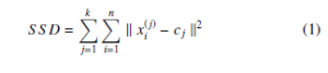
where k x_i^(j) − c_j k² is a L2 norm between a data point x_i^(j) and the cluster center c_j. In AP [30], at the initial stage, all data points are considered as centroids and nodes of the network. The clusters and their centroids are measured by transmitting the similarity message recursively. The Mini Batch k-Means (MBKM) [31] is an improved version of k-means, which performs clustering on batches instead of considering each point. Therefore, MBKM requires less computational time and is also applicable to large datasets.

In hierarchical clustering, groups are formed by iteratively dividing the data objects either in the bottom-up or top-down approach. The bottom-up approach is also known as Agglomerative Hierarchical Clustering (AHC) [22], in which initially each data object is considered as a separate group, then merging these small groups into larger and larger groups until a single group formation or certain threshold. The top-down approach is also known as Divisive Hierarchical Clustering (DHC), and it works in reverse order of the bottom-up approach. Both hierarchical approaches depend on the linkage criteria such as single, complete and average linkage. The linkage criteria determines the metric for merging two similar characterized small clusters. For example, single linkage criteria determines the minimum distance pair from the neighbor clusters minⁿd(x,y) : x ∈ C_i,y ∈ C_j^o. The BIRCH [23] method has proposed to deal with large datasets, outliers in robust and also to reduce the computational complexity. The BIRCH method works on the idea of Cluster Features (CF) which is a height-balanced tree.

The basic idea of fuzzy theory-based clustering is that the discrete labeling is converted to continuous intervals, to describe the belonging relationship among objects more reasonably. The Fuzzy c-means (FCM) [24] is an extension of k-means where each data point can be a member of multiple clusters with membership value. The main advantage of FCM is that the formed groups are more realistic.

The density-based clustering finds the clusters based on the density of data points in a region. The principal objective of densitybased clustering is that for each instance of a group, there should be at least a minimum number of neighbor instances within the given radius. The DBSCAN [25] is the most well known density-based clustering. In DBSCAN clustering, the data objects fall into three groups: core-object, border-object and noise-object. The data points of the core-object group have enough number of neighbors in the given radius, and these data points are from the higher density region. The data points of the border-object group have fewer neighbors than the required number of neighbors in the given radius and they are in the neighborhood of the core object group. The data points of the noise-object group are not in either core or border-object group. The advantage of DBSCAN clustering is that the generated clusters are in arbitrary shape based on the given parameters such as radius and number of minimum instances. The improved version of DBSCAN is OPTICS [26], which overcomes the limitations of DBSCAN. Mean-shift [27] algorithm determines the mean of offset of the current data point, the next point is identified based on the current point and the offset. The process will continue until some criteria is satisfied.

The spectral clustering [28] is a graph partition-based technique in which clustering is obtained by similarity graph partition. The paper [28] describes the different ways of constructing the similarity graph. While building the similarity graph, the data objects are considered as vertices and the similarity (i.e., the similarity distance) between the data objects is a weighted edge. The critical idea of similarity measure is to find a method of graph partition by making edges between different groups have low edge weight and the edges of the same group have more edge weights. In similarity graph partitioning, the cluster analysis is carried out by feature space obtained by the eigenvectors corresponding to k largest eigenvalues of the laplacian matrix [38] of similarity graph. The spectral clustering is suitable for the datasets with arbitrary shape, high-dimensions and outliers.

The EMGMM [29] is a model as well as a distribution-based clustering technique in which cluster data obey the same independent Gaussian distribution which exists in the original data distribution. The generated clusters are more realistic because a probability distribution obtains them.

The performance and applicability of clustering depends on the used dataset characteristics. Therefore, the researchers empirically state that none of the clustering technique is generalized for any datasets.

2.1.2     Cluster validation Measures

In our experimentation, we have used two internal and one external cluster validation measure to evaluate the performance of clustering techniques. The internal measure computes the performance of clustering without using the ground-truth class labels. The compactness (CP) [33] is an internal cluster validation measure which can be computed as follows

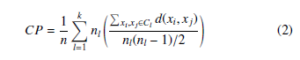
where d(x_i, x_j) is Euclidean distance between two objects in cluster C_l and n_l is the number of objects in C_l. The smaller CP value of clustering is more compact and gives better clustering results. The Calinski-Harabaz Index (CHI) [33] or Variance Ratio Criterion is defined as the ratio of between-clusters dispersion mean and the within-cluster dispersion mean. The CHI is an internal cluster validation measure which is given by

Where n is the dataset size, C is the dataset center, n_l is the size of l^th cluster, C_l is the l^th cluster centroid and NC is the number of clusters.

The external validation measure knows the ground truth class labels. The primary purpose of the external validation index is to choose an optimal clustering algorithm for a given dataset. The external validation measure also checks the cluster purity. In our experiment, we used Fowlkes-Mallows Index (FMI) [32] is the geometric mean between precision and recall. The FMI defined as follows

The FMI value is bounded between 0 and 1, 1 denotes that the obtained clusters and the given ground truth classes are the same. The large FMI indicates that the obtained clustering is purer.

We also measured the contingency matrix that reports the intersection cardinality for every true/predicted cluster pair. The contingency matrix gives sufficient statistics for all clustering metrics. But it is hard to interpret the contingency matrix of extensive clustered data.

2.2        Student t-Distributed Stochastic Neighbor Embedding (t-SNE)

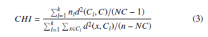
The t-SNE [9] algorithm introduced by Laurens Van Der Maaten and Geoffrey Hinton in 2008, based on the SNE algorithm. The principal objective of SNE is to preserve the underlying structure of high-dimensional data in low-dimensional embedding space. Lets assume the given input data X = {x₁, x₂,….., x_N} where each x_i ∈ R^D is a D-dimensional vector. The t-SNE computes the embedding Y = {y₁,y₂,….,y_N} of X where each y_i ∈ R^d is a d-dimensional vector, where d  D and most commonly d =2 or 3. The similarity between x_i and x_j of X is calculated by conditional probability p_ij is given by

where the bandwidth σ_i of Gaussian kernel, is obtained by binary search by matching the perplexity of P_i and the user-defined perplexity (µ) which is given as a parameter. The perplexity is a smooth measure of an adequate number of neighbors for each data point. The equality and perplexity of P_i is as follows

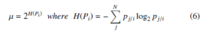
where H(P_i) denotes the entropy and P_i is the conditional probability distribution across all data points for the given x_i. The y_i and y_j are the corresponding low-dimensional values of x_i and x_j (i.e., the values of Y are initialized by Gaussian or uniform distribution).

The similarity between y_i and y_j is defined as

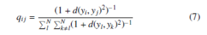
where d(y_i,y_j) is defined as distance similarity measure such as Euclidean distance. In low-dimensional embedding, the similarity q_ij is obtained by student t-distribution with one degree of freedom. But, the similarity p_ij of high-dimensional data uses the Gaussian distribution. The cumulative function curvature of Gaussian distribution is flatter than the cumulative function curvature of student t-distribution with one degree of freedom. The principal idea of using student t-distribution in low-dimensional embedding is to overcome the crowding problem [7].

If p_ij ∼ q_ij, ∀_i,j ∈ N, then the given data is perfectly embedded into the low-dimensional space. Otherwise, compute the KL-divergence (i.e., error) between p_ij and q_ij that is equal to the cross-entropy in Information Retrieval System (IRS). The cost function (C) or objective of t-SNE is defined as follows

The simple gradient descent applied on cost function C for obtaining the optimization or minimization of it. The simple gradient descent of cost function C given by

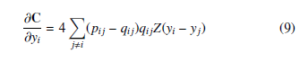
where Z = (1 + d(y_i,y_j)²)⁻¹ is a normalization term of student tdistribution. The Equation 9 produce either positive or negative values depending on the p_ij value. If an Equation 9 gives positive value then there is an attractive force among the y_i and y_j of embedding space. Otherwise, there is a repulsive force among the y_i and y_j of embedding space. The degree of repulsion depends solely on the closeness of points in the embedding space. In the optimization process, the early exaggeration coefficient α > 1 plays a paramount role in forming groups of similar objects of high-dimensional data in low-dimensional embedding space. In the early exaggeration process, the elements of similarity matrix (P) (i.e., p_ij’s) multiplied by the early exaggeration coefficient, which is measured by the intuition given by George C. Linderman and Stefan Steinerberger [39]. Therefore, similar data objects bring near to each other in low-dimensional embedding space. This process can happen at the early stage of optimization. The gradient descent of C after early exaggeration is

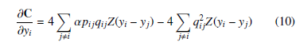
The momentum and learning rate parameters improve the optimization process of the cost function. The momentum parameter reduces the number of iterations of the cost function optimization. At the initial stage of iteration, the momentum value is small until the map points have become moderately well organized. The optimization is improved by input approximation and tree-based algorithms [13], which reduce the memory and computational complexity. The updated values of Y at iteration t is obtained by

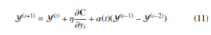
where α(t) is momentum at t^th iteration, η is learning rate. The work-flow of t-SNE is shown in the Figure 1.

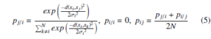
The well-separated clusters of input data are well preserved in the low-dimensional embedding by setting the early exaggeration coefficient α and learning rate η. The intuition for setting the above parameter is derived by George C. Linderman and Stefan Steinerberger in [39]. According to the George C. Linderman and Stefan Steinerberger observations the early exaggeration coefficient α, learning rate η, and minimum probability p_ij’s of same cluster objects(i.e., x_i and x_j belong into the cluster C_l for all i , j) is defined as follows.

where π : {1,2,….,n} → {1,2,…,k} assigns each data point to one of the k clusters.

2.3        Local Inverse Distance Weighting Interpolation (LIDWI)

The LIDWI [40] maps new data point x ∈ R^D into the existing embedding y_i ∈ R^d, where {i = 1,2,…….m}. The LIDWI determines the value of x as a weighted sum of values y_i, where weight is proportional to inverse distances. The LIDWI of x is

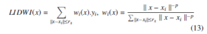
for instance, when the data point x → x_i, the inverse distance k x − x_i k⁻¹→ ∞, the corresponding weight w_i(x) → 1 ( i.e., ∀_j,iw_j(x) → 0 due to the normalization) and LIDWI(x) → y_i. The neighbor points selection is obtained by a radius r_x parameter. The parameter r_x value is calculated by the heuristic proposed by Andrey Boytsov et.al. [17]. In LIDWI, the power parameter p plays an important role. For instance, very small value of p predicts the value of x around the center: y ≈ mean(y_i) (unless x = x_i) even the distance k x − x_i k is low because the weight distribution is close to uniform. When the power parameter is high and the distance k x − x_i k is low, the weight w_i(x) of very first nearest neighbor is dominating all other neighbors, therefore y ≈ y_i where i = argmin k x − x_j k. The overfitting suffers from either too small or too large values of power parameter p. In LOIN-tSNE, the authors proposed a generalization for obtaining power parameter by using leave-one-out cross-validation of the training sample. The computation of the generalized power parameter is obtained by applying the LIDWI for each training sample that produces the estimation of each y_i. Then the mean square distance between the estimated y_i’s and real y_i’s is computed. The optimal power parameter is obtained by optimizing the mean square error (i.e., the mean square distance is minimum). The obtained power parameter is considered as a metric. However, this metric is heuristic, not an exact criterion.

2.4        Performance evaluation metrics

2.4.1     k-NN accuracy

The existence of the cluster structure of high-dimensional data in low-dimensional embedding is quantitatively measured by k-NN accuracy of the t-SNE embedding in the context of clustering. The k-NN accuracy is defined as the percentage of the neighbors having the cluster label equivalent to the observational point cluster label.

2.4.2     Trustworthiness

Trustworthiness [41] is one of the measure to evaluate the quality of the t-SNE embedding. Trustworthiness is defined as any unexpected nearest neighbors in the output space are penalized in proportion to their rank in the input space.

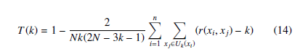
where U_k(x_i) is the k-NN of x_i in embedding space, r(x_i, x_j),i , j the rank of x_j when the data vectors are ordered based on their Euclidean distance from the data vector x_i in the original data space. It is bounded between 0 and 1, where 1 represents the complete structure of the data preserved in the embedding space.

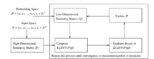
Figure 1: Work-flow of t-SNE algorithm [19]

3. Related Work

Our earlier proposed k-NN sampling based tSNE mainly concentrates on the preservation of the underlying structure of highdimensional data in low-dimensional embedding space with representative samples. The obtained low-dimensional embedding structure describes the quality of the structure using ground-truth class labels. But the low-dimensional embedding does not give the quantitative proof for the number of clusters that exist in the original data. In [39] authors gave the theoretical observations for well-separated clusters of high-dimensional data in low dimensional embedding space.

The researchers have proposed various methods to incorporate new data samples into the existing t-SNE environment. Most of the existing techniques designed a mapping function f : X → Y, which accepts multi-dimensional data and returns its low-dimensional embedding. The designed mapping functions are used for incorporating the new data samples into the existing t-SNE environment. In [14–16] authors have proposed different approaches for adding a new data sample or scaling up the t-SNE algorithm.

Andrey Boytsov et.al. [17] proposed the LION-tSNE algorithm based on local IDWI for adding new data sample into an existing tSNE environment. It also addresses the outlier handling approaches. Our earlier work extended the idea of the LION-tSNE algorithm by proposing a k-NN sampling method for designing a representative sampling based t-SNE model. It allows the selection of the sample concerning their k-nearest neighbors instead of random sampling. In this paper, we are proposing the novel representative k-NN sampling-based cluster approach for effective dimensionality reduction-based visualization of dynamic data, which determines the underlying cluster by using the most popular clustering techniques. The obtained cluster structure is quantitatively evaluated by k-NN accuracy in the context of clustering and trustworthiness.

4. Proposed representative k-NN samplingbased clustering for effective visualization Framework

The proposed representative k-NN sampling-based clustering for effective dimensionality reduction-based visualization of dynamic data framework is shown in the Figure 2. It has four phases: at phase 1, data preprocessing is done for removing the redundant data points and filling the empty variables with appropriate values. At phase 2, the proposed k-NN sampling-based clustering is applied to determine: (i) The generation of k distinct samples using mutual k-NN sampling with static graph updation algorithm. (ii) The list of clustering techniques applicable for the given dataset. (iii) The optimal sample size produces the best grouping for each concerned clustering technique. (iv) The ordered sequence of recommended clustering techniques for the given dataset from which the best clustering technique is selected by using FMI scores. The detailed representative k-NN sampling-based is clustering presented in section 4.1. At phase 3, the dimensionality reduction-based visualization is obtained by t-SNE algorithm, which derives the low-dimensional embedding of data and the LIDWI algorithm is used to interpolate the new data points into the learned t-SNE model. The outliers from the remaining data points are identified and controlled by the proposed heuristic. The dimensionality reduction-based visualization is described in section 4.2. In the final phase, the quantitative measure of the t-SNE embedding is computed by k-NN accuracy and trustworthiness. The process of quantitative metric derivation is described in section 4.3.

4.1        Representative k-NN sampling-based clustering

Initially, the k distinct samples are generated by the modified algorithm of our earlier proposed method. The sample generation depends on the parameter k of k-NN sampling. Each k generates one distinct sample; the boundary of k is denoted as 1 ≤ k ≤ m, where m is the maximum number of neighbors required for preserving the behaviour of any data point of the given dataset. Our earlier approach has given two different k-NN sampling strategies LION-tSNE with quantitative measure of cluster accuracy such as static and dynamic k-NN sampling based on k-NN graph modification. In this paper, we are considering only static k-NN sampling in which the k-NN graph is modified statically that means no new edge is added among any two vertices of the k-NN graph. The main reason for selecting static k-NN sampling is that the t-SNE embedding results of it are more statistically significant than the dynamic one. The Nearest Neighbor score (NN score) and Mutual Nearest Neighbor score (MNN score) of each node of the k-NN graph are used for selecting the samples. Lets assume k-NN graph is a directed graph G = (V, E), the edge E(v₁,v₂) gives v₂ as a neighbor of v₁ and neighborhood of v₁ is denoted by N_v1. The out-degree of each vertex is equal to k, and the in-degree of a vertex depends on the neighborhood property of other vertices (i.e., the data point x_i belong into the neighborhood of other datapoints). In our method, each data point is a vertex of the k-NN graph and k is a parameter for deriving the edges between neighboring vertices. The NN score of data point x_i is equal to the in-degree of x_i which is defined as follows

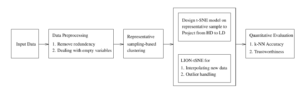
Figure 2: Proposed framework of representative k-NN sampling-based clustering for an effective dimensionality reduction-based visualization of dynamic data using

The updated mutual k-NN sampling with a static graph updation algorithm is shown in Algorithm 1. Initially, the Train samples (i.e., representative samples set) and Rep samples (i.e., the sample represented by the selected training sample that is the first nearest mutual neighbor of train sample) are null sets. For each iteration, the data point x which has maximum NN and maximum MNN score appended to the Train samples set. The data point y is appended to the Rep samples if y ∈ N_x and x ∈ N_y that denotes the point x and y are more similar (i.e., the distance d(x,y) < d(x,z) where ∀z ∈ N_x) to each other. The data point x and y are deleted from X and their corresponding vertices are deleted from the k-NN graph. After deleting the vertices of x and y, the corresponding in-edges and out-edges are removed from the k-NN graph and the graph is updated accordingly. The elements of Train samples and Rep samples are obtained iteratively, the iteration repeats until the NN score of the remaining X is equal to zero.

Algorithm 1: Mutual k-NN Sampling with a static graph updation

Data: data set X = {x₁, x₂,…..x_N}, parameter k for minimal training sample selection

Result: Return Train samples, Rep samples

Train samples = ∅

In our earlier approach of static graph updation, we have considered the whole mutual neighborhood set of x as the samples represented by x. The whole neighborhood set selection causes loss of information due to that reason the earlier approach select Train samples set at an early stage of k value. The data points of the remaining X (i.e., the data point do not belong into either Train samples set or Rep samples set) is handled in two different ways. Handling of the remaining samples is described in subsection 4.4. The mutual k-NN sampling with a static graph updation algorithm generates a various set of Train samples and Rep samples with different k-values.

The clustering techniques which are described in subsection 2.1.1 are applied on each Train samples set of mutual k-NN sampling with a static graph updation algorithm that is called a samplingbased clustering. The cluster labels for the data points other than the Train samples are assigned by using k-NN algorithm. For example, the dataset size is N, the Train samples size is n and then the unmarked sample size is N − n(i.e., the samples are not assigned with any labels). The k-NN of each unmarked sample is derived from the associated Train samples set. The label assignment of each unmarked sample depends on the labels of its k-NN, a label with maximum occurrence in k-NN that is assigned to a sample. From each clustering technique, the optimal Train samples set is obtained by the FMI score. The FMI is an external validation index that uses the ground truth class labels. Therefore, the number of clusters is defined as a constant that is equal to the number of ground truth classes. The FMI score of optimal Train samples of clustering techniques generates an order sequence of the clustering techniques. From the order sequence, we can recommend the most desirable techniques for a given dataset from the selected set of techniques. From this recommendation, the best suitable technique is selected and its optimal Train samples set is considered as the best representative sample. The threshold parameter is used to derive the recommended techniques, which is defined as the FMI score difference between two adjacent techniques of order sequence. The three cluster validation index such as FMI score, CHI score and CP of representative k-NN sampling-based clustering are compared with their aggregate clustering (i.e., clustering on whole dataset) validation index of chosen clustering techniques. The result comparison is discussed in subsection 5.3. The algorithm of representative k-NN sampling-based clustering is shown in Algorithm 2. The embedding of selected optimal Train samples and addition of other data samples into an existing t-SNE environment is described in the following section.

4.2        Dimensionality reduction-based visualization

The subsection 4.2.1 describes the low-dimensional embedding of a representative sample with t-SNE algorithm. Subsection 4.2.2 describes the addition of new data samples into an existing t-SNE environment that is called out-off-sample extension.

4.2.1 Low-dimensional embedding of a representative sample with t-SNE algorithm

Barnes-Hut t-SNE (BH-tSNE) [13] algorithm is an optimized version of the t-SNE algorithm. BH-tSNE optimizes the t-SNE objective function by input similarity approximation and gradient descent approximation. Therefore, it generates low-dimensional embedding of data with minimum computational and memory complexity than original t-SNE. In our approach, the BH-tSNE algorithm is used in two different ways for calculating the low-dimensional embedding space: 1. Baseline t-SNE embedding, 2. Sampled t-SNE embedding. The baseline t-SNE embedding is obtained by applying BH-tSNE on the whole dataset. In contrast, the sampled t-SNE embedding is obtained by applying BH-tSNE on the best representative sample, which is selected from the representative k-NN sampling-based clustering. The Baseline t-SNE embedding results analyze the overall structure of the data in low-dimensional embedding. The sampled t-SNE embedding results analyze the data structure with sampled data and allows the addition of new data samples into an existing t-SNE environment, which solves the scalability issue of the t-SNE. For obtaining a well-separated cluster in low-dimensional t-SNE embedding, the value of early exaggeration coefficient α, learning rate η and input similarity probability p_ij’s are adjusted according to the George C.linderman and Stefan Steinerberger intuition. In our experimentation, the initial solutions of t-SNE is assigned in three different ways, such as random, PCA based and MDS based initial solutions. The random initial solution takes many iterations for convergence. The PCA and MDS based initial solutions overcome the problem of random initialization and they produce better accuracy results, but their initial solution is cost-effective. Adding new data points into a designed t-SNE model is discussed in the below section.

4.2.2    Out-off-sample extension: Interpolation and Outlier handling

The addition of new data point to t-SNE embedding depends on the parameter r_x, r_y and r_close values. The value of parameter r_x, r_y and r_close is obtained from the best representative sample and the t-SNE embedding of it. The parameter r_x is defined as the percentile of the 1-NN distance of a representative sample that decides whether the given new data point is either inlier or outlier. In our proposal, we came to know that the objects of the representative sample set are representing at least one sample of the dataset. Therefore, the representative sample set does not contain any outlier object and we have considered the parameter r_x as the maximum 1NN distance of it. If the new data point x has at least one data point within the r_x from the representative sample set, then x is an inlier, otherwise outlier. The dilation factor (df) is used to derive a heuristic r_x = (1+d f) ∗ r_x which controls the consideration of outliers percentage. The LIDWI interpolation technique is used for adding an inlier data point to the t-SNE embedding of the representative sample set. The outlier placement depends on the parameter r_y and r_close. The outliers placed into the t-SNE embedding of the representative sample set according to the heuristic of Boytsov et.al. [17]. The k-NN accuracy and trustworthiness of t-SNE embedding quantitatively evaluate the existence of a high-dimensional cluster in the low-dimensional embedding. The quantitative evaluation described in the following section.

4.3        Quantitative metric derivation: k-NN accuracy

In our experimentation, the k-NN accuracy is calculated in two different ways: baseline accuracy and sampling accuracy. The kNN accuracy of t-SNE embedding of aggregate data is known as baseline accuracy. The sampling accuracy is computed in three different forms such as training accuracy, test accuracy and overall accuracy. The k-NN accuracy of t-SNE embedding of the representative sample is known as training accuracy. The k-NN accuracy of interpolated samples (i.e., the samples other than the representative sample) is known as test accuracy. The k-NN accuracy of combined low-dimensional space (i.e., the integration of t-SNE embedding of sampled data and interpolated data) is known as overall accuracy. The k-NN accuracy typically depends on the parameter k, which is considered as fixed in our experimentation which is discussed in subsection 5.2. For instance, the smaller k will give good performance accuracy and while increasing the k, performance accuracy will decrease. The selection of parameter k also plays a paramount role in k-NN accuracy measure. The relationship between the parameter k and accuracy is shown in the Figure 3. For quantitative performance evaluation, the k-NN accuracy of representative k-NN samplingbased clustering and aggregate clustering are compared with the k-NN accuracy of ground truth class labels, which is discussed in subsection 5.3.

4.4        t-SNE sample selection criteria

In our experimentation, we have considered two different sample selection criteria for designing the t-SNE model. In the first criteria, the samples are mostly representative of at least one or more other samples. The samples are obtained by a mutual k-NN sampling with a static graph updation algorithm and the best representative sample is selected by the representative k-NN sampling-based clustering. We observe that most of these samples were chosen from the dense region because they produce good NN score and MNN score.

Therefore, these samples do not contain any outliers. In this criterion, the outliers from the remaining sample addition are not sufficiently identified by the adequate 1-NN distance. The outliers consideration is controlled by the proposed heuristic, which is discussed in subsection 4.2.2. In the second criteria, the data points added to the representative sample from the remaining data points using (t,m, s)-Nets sampling [42]. For the addition of (t,m, s)-Nets samples, we used the same procedure of our earlier work. The (t,m, s)-Nets select samples randomly in a uniform distribution. These samples may not represent any other samples and the samples may change among the executions due to the randomness. Therefore, the samples of this criteria may contain outliers. The outliers of this criteria are handled in similar ways as they are handled in our earlier approach.

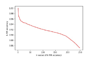
Figure 3: Relationship between k-value of k-NN accuracy and k-NN accuracy which is obtained from the baseline accuracy of k-NN sampling-based clustering.

5. Experimental result analysis

Here we are briefing the datasets, experimental setup and the result analysis. Section 5.1 describes the numerical datasets of different characterizations. The details about the experimental setup is given in section 5.2. The results analysis of each dataset is described in section 5.3.

5.1        Datasets

In our experimental evaluation, we have considered differently characterized datasets such as IRIS, Breast-Cancer, Leukemia, Wine, MNIST, Olivetti-Faces, and COIL-20. The Table 1 provides a detailed description of all the datasets which are downloaded from the UCI Machine Learning repository [43]. For our experimentation, the features of IRIS, Breast-Cancer and Wine datasets are normalized between zero and one, which improves the computational complexity. Initially, the KernelPCA [44] is applied to reduce the dimensionality of the high-dimensional datasets such as Leukemia, MNIST, Olivetti-Faces and COIL-20. The Leukemia dataset is a micro-array of gene expression. The MNIST, Olivetti-Faces and COIL-20 are image datasets that are represented in pixel orientations. The MNIST is a handwritten digits dataset. The Olivettifaces dataset consists ten face images of 40 individuals with small variation in viewpoint, the addition of glass and large variation in expression. The COIL-20 is an image of 20 group objects such as animals, furniture and etc.

Table 1: Overview of datasets along with their size, dimensions, and classes

Dataset Name	Size	Dimensions	# Classes
IRIS	150	4	3
Breast Cancer	569	30	2
Leukemia-ALL-AML	72	7129	2
Wine	178	13	3
MNSIT	70K	784	10
Olivetti faces	400	10304	40
COIL-20	1440	1024	20

5.2        Experimental configuration

In our experimentation, The parameter k of Algorithm 1 is initialy considered as 1 ≤ k ≤ 50. The upperbound of k is equal to largest perplexity value from the literature study [9]. The perplexity is set between 5 and 50 for a fairly good visual representation of any real-world data. In our proposal, the samples of any clustering technique depends on the parameter k. Also, we observed that when there is an increment in parameter k then there is an increment or no change in FMI score of clustering until certain k value. The FMI score becomes stable afterwards. In our experimentation at most of the cases, the selected clustering technique generates representative sample with k value less than or equal to 20. In other cases, the cluster technique generates representative sample with k value greater than 20. But there is an small increment in FMI score comparatively FMI score of clustering with k value less than or equal to 20. Therefore, we have generalized the k-value as less than or equal to 20. The sensitivity of parameter k needs to be investigated more in future. The number of clusters is defined as a constant that is equal to the number of ground truth classes. The original class labels are not used anywhere in the experimental evaluation. The ground truth class labels are used only for measuring the FMI score that determines the cluster purity. The threshold parameter is set to 0.05 that provides the intuition for selecting the recommended clustering techniques from the order sequence. The threshold parameter derived from the statistical method where the maximum allowable difference between two consecutive values of either increasing or decreasing order sequence is 5%. The recommended set size and threshold parameters are inversly proposional to each other. The sensitivity of threshold parameter needs to be investigated further. From the recommended set, the best technique is chosen and the optimal sample of it being considered as the best representative sample for designing the t-SNE model. The representative sample is embedded in a 2D space using the BH-tSNE algorithm. The parameters of BH-tSNE are set up according to the paper [13] experimental setup. In addition to that, we initialized the embedding space Y by sampling the point y_i from a uniform distribution with [−0.02,0.02]² for obtaining well-separated clusters in embedding space. The datasets with more than 50 dimensions, their dimensionality is reduced to 50 by kernel PCA. The dimensionality reduction speeds up the computation of the probability distribution of the input similarity and suppresses some noise. The results of the BH-tSNE algorithm are shown in 2D scatter-plot representation. The minimum value of p_ij of clustered data, the early exaggeration factor α and the learning rate η values are assigned similar to the George C.linderman and Stefan Steinerberger paper.

The data points other than the representative samples are interpolated into the BH-tSNE of a representative sample using LIDWI. The parameter r_x is obtained by either proposed heuristic or intuition of LION-tSNE. In the proposed heuristic dilation factor is bounded between 0 and 1. The parameter r_y, r_yclose and power are measured similar to LION-tSNE algorithm.

Table 2: Parameters setting for the experimental setup

Parameter	Value
k of k-NN sampling	1
Threshold	0.05
Perplexity	5 – 50
Early exaggeration coefficient Adaptive learning rate	1
Dilation Factor	0
rx at dist perc ry at dist perc ryclose at dist perc Fixed k-value for k-NN accuracy	3 – 10

Table 2 provides the parameter settings of our experimental evaluation. The parameter perplexity represents the effective number of neighbors for each data point. For instance, the small value of perplexity creates subgroups within the same cluster of t-SNE results. In contrast to small, the large value of it does not maintain the clear separation between two clusters of t-SNE results. Both cases suffer from either under-fitting or over-fitting problem that causes a lack of visual clarity. The empirical studies state that the perplexity value between 5 to 70 gives a good visual representation of t-SNE results. The parameter dist per represents the overall percentile of the representative sample that needs to be considered as inliers. For example, if we take dist per as 95th percentile, that means out of 100 points, 95 points are considered as inliers and the remaining 5 points are outliers. The parameter k plays an important role in the computation of k-NN accuracy of the data. The effect of parameter k is shown in the Figure 3. It is clear that when there is an increment in k value, accuracy decreases monotonically. The result evaluation of representative k-NN sampling-based clustering is discussed in the next section.

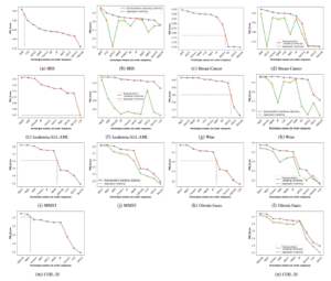
Figure 4: The column one and column three (i.e., sub-figure ((a), (c), (e), (g), (i), (k) and (m)) shows the threshold derivation (i.e., the integration of doted horizontal and vertical lines) of all seven datasets from the order sequence curve. The column two and column four (i.e., sub-figure (b), (d), (f), (h), (j), (l) and (n)) shows the relationship curve of all datasets from the order sequence, which provides the relationship between the FMI scores of proposed representative k-NN sampling-based clustering and

5.3        Result analysis

In our experimentation, we have considered most frequently and popularly used clustering techniques. The Figure 4 shows the curves of all seven datasets of subsection 5.1. The Figure 4 gives the threshold derivation for the recommended order sequence and relationship between the FMI scores of proposed representative k-NN sampling-based clustering and aggregate clustering. In the Figure 4, the x-axis represent the clustering technique names in the order sequence of FMI scores (i.e., FMI(t₁) > FMI(t₂) > …. > FMI(t_l) where t_i represents i^th best clustering technique) and y-axis represents the corresponding FMI Scores. Column one and column three of Figure 4 (i.e., sub-figure (a), (c), (e), (g),(i), (k) and (m)) shows the threshold derivation for the recommendation of clustering techniques for all the given seven datasets. The column two and column four of Figure 4 (i.e., sub-figure (b), (d), (f), (h), (j), (l) and (n))

Table 3: The applicable clustering and their recommended order sequence for the given seven datasets. Dataset Applicable cluster methods Recommended order sequence of cluster methods IRIS k-Means, Agglomerative, BIRCH, Spectral, EMGMM, FCM, DBSCAN, AP, MBKM, OPTICS, MS EMGMM Breast-cancer k-Means, Agglomerative, BIRCH, Spectral, EMGMM, FCM, DBSCAN, AP, MBKM, OPTICS, MS EMGMM, BIRCH, k-Means, MBKM, FCM, Agglomerative, AP, Spectral Leukemia k-Means, Agglomerative, BIRCH, Spectral, EMGMM, FCM, DBSCAN, AP, MBKM, OPTICS MBKM, EMGMM, DBSCAN, AP, k-Means, BIRCH, Agglomerative, OPTICS, Spectral, FCM Wine k-Means, Agglomerative, BIRCH, Spectral, EMGMM, FCM, DBSCAN, AP, MBKM, OPTICS, MS Agglomerative, Spectral, MBKM, AP, FCM, k-Means, EMGMM, MS, OPTICS MNIST k-Means, Agglomerative, BIRCH, Spectral, EMGMM, FCM, DBSCAN, AP, MBKM, OPTICS BIRCH, Agglomerative, EMGMM, k-Means, AP, MBKM Olivetti-faces k-Means, Agglomerative, BIRCH, Spectral, EMGMM, FCM, DBSCAN, AP, MBKM, OPTICS BIRCH, Agglomerative, k-Means, EMGMM, MBKM, AP COIL-20 k-Means, Agglomerative, BIRCH, Spectral, EMGMM, FCM, DBSCAN, AP, MBKM, OPTICS DBSCAN, Agglomerative

shows the relationship curve that provides the relationship between the FMI Score of representative k-NN sampling-based clustering and aggregate clustering for all the given seven datasets. The Figure 4 clearly shows that the proposed representative k-NN samplingbased clustering results are superior to the aggregate clustering results.

The sets of applicable and recommended order sequence of clustering techniques for the given seven datasets is listed in the Table 3. The CP and HCI of representative k-NN sampling-based clustering and aggregate clustering of all clustering techniques are listed in the Table 4 and 5. The Table 4 and 5 clearly states that the CP of the proposed representative k-NN sampling-based clustering is smaller than the aggregate clustering for some techniques. In contrary techniques, the compactness is in reverse order, but the compactness difference is very minute in both situations. The CHI is also deriving the relationship between both clustering as same as CP where the CP is small, and then there is a large CHI score.

The contingency matrices of representative k-NN samplingbased clustering and aggregate clustering of IRIS, Wine, Breastcancer and Leukemia datasets are shown in the Table 6, 7, 8 and 9. If the number of classes of the given dataset is larger, then it is difficult to analyze the data with the contingency matrix. Therefore, the contingency matrix of MNIST, Olivetti-Faces and COIL-20 datasets are not addressed. The Table 6, 7, 8 and 9 clearly states that the proposed representative k-NN sampling-based clustering classifies the labels much similar to the ground truth class labels compared to aggregate clustering. The Tabel 9 represents the contingency matrix of the Leukemia dataset, which indicates that none of the selected technique gives the best clustering results. Still, representative k-NN sampling-based clustering produces better results than the aggregate clustering.

For Quantitative evaluation, the baseline k-NN accuracy of proposed representative k-NN sampling-based clustering is compared with baseline k-NN accuracy of aggregate clustering and baseline k-NN accuracy of ground truth class labels. The baseline k-NN accuracy and trustworthiness of representative k-NN sampling-based clustering, aggregate clustering and ground truth class labels of seven datasets are listed in Table 10. The Table 10 clearly indicates that the proposed method produces more robust results than others.

Table 4: Compactness and CHI score of representative k-NN sampling-based clustering, overall sampling clustering (i.e., assigning the cluster labels based on the KNN of remaining samples in the context of representative samples) and the aggregate clustering of IRIS, Breast-Cancer, Leukemia and Wine datasets for the selected clustering techniques.

Method	Samp. size	Compactness			CHI Score
		Samp. cltr	Overall cltr	Aggr. cltr	Samp. cltr	Overall cltr	Aggr. cltr
k-Means	73	0.4945	0.5601	0.5557	221.54	347.56	358.56
Agglomerative	63	0.5143	0.5579	0.5606	178.78	353.21	348.03
Birch	73	0.5291	0.5646	0.8507	183.85	335.22	193.97
Spectral	60	0.5234	0.5606	0.5709	167.457	348.03	322.48
EMGMM	63	0.5316	0.5754	0.5789	161.44	317.59	307.76
FCM	72	0.5107	0.5633	0.5576	197.71	340.79	355.71
DBSCAN	73	0.6379	0.7047	0.6723	104.84	175.96	124.78
AP	73	0.52	0.557	0.5588	196.99	354.54	353.22
MBKM	74	0.4834	0.5613	0.5562	234.32	343.95	356.28
OPTICS	73	0.5894	0.6071	1.0919	120.53	259.45	15.99
MS	70	0.527	0.557	0.6002	188.2	354.45	289.52
Breast-Cancer
k-Means	291	1.5608	1.6064	1.6013	203.91	355.42	364.09
Agglomerative	290	1.5735	1.6073	1.6322	199.73	356.80	319.01
Birch	291	1.5698	1.6083	1.9509	193.53	352.67	53.96
Spectral	289	1.5694	1.6177	1.6449	197.34	351.45	328.74
EMGMM	276	1.5744	1.6096	1.6168	178.38	350.08	337.00
FCM	276	1.5645	1.6048	1.6001	186.30	358.22	363.04
DBSCAN	291	1.9493	2.0004	1.9735	21.27	19.66	38.11
AP	213	1.5146	1.6088	1.6088	156.95	356.82	358.62
MBKM	268	0.8824	1.6047	1.6007	180.883	359.63	363.83
OPTICS	268	1.9635	2.0179	2.0069	21.72	24.65	38.41
MS	213	1.9138	2.0054	1.9412	19.79	17.65	68.97
Leukemia-ALL-AML
k-Means	22	3.4413	3.9367	3.9279	1.567	1.173	1.685
Agglomerative	19	3.3494	3.9315	3.9222	1.874	1.269	1.756
Birch	19	3.3494	3.9315	3.919	1.874	1.269	1.921
Spectral	19	3.3076	3.915	3.92	1.707	1.279	1.845
EMGMM	20	3.4012	3.9415	3.9237	1.337	0.953	1.591
FCM	20	3.3743	3.939	3.9271	1.622	1.117	1.619
DBSCAN	17	3.2654	3.9436	3.9225	1.351	0.959	1.326
AP	14	2.8993	3.895	3.9355	1.548	0.882	1.292
MBKM	22	3.3088	3.8957	3.9366	1.102	0.859	1.122
OPTICS	19	3.315	3.922	3.9071	0.859	0.717	1.317
MS	…	….	….	….	….	….	….
Wine
k-Means	82	1.3275	1.4298	1.4289	47.255	82.828	83.373
Agglomerative	87	1.3207	1.4356	1.4328	45.964	80.465	81.327
Birch	82	1.555	1.6567	1.629	19.859	34.395	42.564
Spectral	87	1.3532	1.4348	1.4298	42.372	81.014	82.828
EMGMM	71	1.3481	1.4331	1.4348	39.846	81.796	81.698
FCM	85	1.3473	1.4317	1.4305	45.029	82.346	83.135
DBSCAN	64	1.6181	1.6656	1.9606	15.719	37.502	3.102
AP	82	1.5534	1.3368	1.4458	45.362	80.714	80.828
MBKM	87	1.3562	1.4848	1.4278	42.472	81.784	81.523
OPTICS	85	1.4484	1.4531	1.4248	38.866	82.796	81.698
MS	71	1.3489	1.4371	1.4748	49.846	81.797	80.598

Table 5: Compactness and CHI score of representative k-NN sampling-based clustering, overall sampling clustering (i.e., assigning the cluster labels based on the KNN of remaining samples in the context of representative samples) and the aggregate clustering of MNIST Handwritten digits, Olivetti-Faces and COIL-20 datasets for the selected clustering techniques.

MNIST

Method	Samp. size	Compactness			CHI Score
		Samp. cltr	Overall cltr	Aggr. cltr	Samp. cltr	Overall cltr	Aggr. cltr
k-Means	4481	3816.4	3897.8	3877.8	233.97	477.45	492.48
Agglomerative	4900	3936.2	3974.2	3974.2	206.16	409.22	395.43
Birch	4900	3936.2	3974.2	3974.2	206.16	409.22	395.43
Spectral	4735	4662.2	4694.5	4695.0	1.048	1.0308	1.0459
EMGMM	4206	3862.2	3930.6	3977	200.8	443.59	400.32
FCM	4835	3962.2	4374.5	4555.	1.248	1.308	1.59
DBSCAN	4735	4662.2	4694.5	4695.	1.048	1.0308	1.0459
AP	4496	3832.5	3978.6	3897.3	213.97	457.78	472.34
MBKM	4783	4216.4	4597.1	4577.3	224.17	467.65	452.18
OPTICS	4625	3962.5	4094.3	4195.7	1.258	1.13	1.045
MS	…	….	….	….	….	….	….
Olivetti-Faces
k-Means	200	1568	1784.5	1565.8	10.384	14.009	21.210
Agglomerative	178	1495.9	1798.8	1546.8	10.718	13.634	22.008
Birch	178	1495.9	1798.8	1546.8	10.718	13.634	22.008
Spectral	188	2235	2545.9	2608.4	0.6858	0.6839	0.9924
EMGMM	165	1528.9	1812.8	1591.5	9.211	13.168	20.272
FCM	178	2479.3	2659.4	2732.6	4.321	4.874	4.178
DBSCAN	194	2679.4	2750.5	2745.1	4.021	3.804	5.782
AP	194	1628.9	1852.8	1691.5	10.321	14.168	20.872
MBKM	178	1668.6	1852.8	1671.5	9.711	12.168	21.275
OPTICS	165	1598.4	1932.8	1891.5	8.217	13.468	22.728
MS	…	….	….	….	….	….	….
COIL-20
k-Means	679	10.333	10.362	10.180	87.911	183.571	188.454
Agglomerative	701	10.239	10.237	10.294	90.220	184.703	181.461
Birch	701	10.577	10.562	11.1165	87.377	180.283	162.538
Spectral	676	14.852	14.944	17.447	28.585	57.964	27.4288
EMGMM	679	10.273	10.243	10.356	87.832	186.73	187.686
FCM	689	12.872	13.645	15.745	34.784	56.768	34.58
DBSCAN	679	18.843	18.962	19.769	19.532	38.902	38.548
AP	701	10.573	10.253	10.856	83.83	188.63	186.656
MBKM	679	10.253	10.143	10.366	80.832	188.73	187.656
OPTICS	679	10.243	10.233	10.326	87.432	185.738	184.286
MS	…	…	…	…	…	…	…

Table 6: Contingency matrix of k-NN sampling-based and original clustering on IRIS dataset with best k-NN sampling-based clustering technique (i.e., EMGMM).

Class labels generated by

k-NN samplingbased clustering	Aggregate clustering
C1         C2             C3	C1         C2         C3
50          0           0	50          0           0
0            49         1	0            45         5
0            2                48	0            0           50

Original

Table 7: Contingency matrix of k-NN sampling-based and original clustering on Wine dataset with best k-NN sampling-based clustering technique (i.e., Agglomerative).

Class labels generated by

k-NN samplingbased clustering	Aggregate clustering
C1          C2             C3	C1          C2         C3
0            0                59	2            0           57
69          2            0	69          2            0
1            47          0	0            48          0

Original

The sampling k-NN accuracies such as train, test and overall of t-SNE embedding of a representative sample and interpolation of other samples are listed in Table 11 and the overall trustworthiness is also covered. The best representative sample of representative k-NN sampling-based clustering and random sampling of IRIS dataset is shown in Figure 5. The 2D scatter-plots shown in Figure 5 are the first two coordinates of IRIS dataset. The Figure 5(a) shows the best representative sample of k-NN sampling and the Figure 5(c) shows the representative sample of k-NN sampling along with samples of (t,m,s)-Nets of remaining data points. The Figure 5(b) and 5(d) shows the random sampling of size equal to the sample size of Figure 5(a) and 5(c). The samples of Figure 5(a) are constant and consistent comparatively other sampling.

Table 8: Contingency matrix of k-NN sampling-based and original clustering on Breast-Cancer dataset with best k-NN sampling-based clustering technique (i.e., EMGMM).

Class labels generated by

k-NN samplingbased clustering	Aggregate clustering
C1          C2	C1          C2
21         191	16         196
352       5	340       17

Original

Table 9: Contingency matrix of k-NN sampling-based and original clustering on Leukemia dataset with best k-NN sampling-based clustering technique (i.e., MBKM). Class labels generated by

k-NN samplingbased clustering	Aggregate clustering
C1         C2	C1         C2
0           47	9           38
2           23	6           19

Original

Table 10: Baseline k-NN accuracy of k-NN sampling based clustering, original clustering and ground truth class labels

Dataset Name	Trust		Baseline k-NN Accuracy
		Sampling Clustering	Aggregate Clustering	Ground-truth class labels
IRIS	0.9861	0.9735	0.9666	0.96
Breast-Cancer	0.958	0.9876	0.9862	0.9577
Leukemia	0.6799	0.9875	0.6643	0.7485
Wine	0.9552	0.9774	0.9828	0.9717
MNIST Digits	0.9895	0.9259	0.9483	0.9512
Olivetti face	0.9494	0.6775	0.8287	0.88
COIL-20	0.9972	0.9554	0.9709	0.9743

The Figure 6 shows the 2D scatter-plot visualization of IRIS data with outliers projection. In Figure 6, we are also showing the outliers (i.e. denoted by large grey color circle) of original data after finding the outliers from the addition of remaining data points with the radius r_x which is obtained by the proposed heuristic r_x = (1 + d f) ∗ r_x with d f = 0.2. It clearly states that sampled data obtain the outliers of original data.

The 2D scatter-plot visualization of embedding space of representative k-NN sampling-based clustering of the MNIST dataset is shown in the Figure 7. The Figure 7 shows the baseline 2D scatter-plot of t-SNE embedding of whole MNIST data of size 10K

Table 11: Quantitative measure using k-NN accuracy of k-NN sampling based clustering, original clustering and ground truth class labels Optimal Sample Dataset                                Sample           Trust                                                                                                        Sampling k-NN Accuracy Name Size Sampling-based clustering   aggregate clustering Ground truth class labels     Train Test Overall Train   Test Overall Train Test Overall IRIS 73 0.9594 0.9726 0.9594 0.9661 0.9753   0.9405 0.9652 0.9589 0.9324 0.9585 Breast Cancer 291 0.9239 0.9896 0.9856 0.9820 0.9690   0.9856 0.9876 0.9452 0.9676 0.9546 Leukemia 33 0.5665 0.9416 1.0 0.9875 0.6714   0.4102 0.6266 0.6363 0.5897 0.6247 Wine 87 0.9299 0.9377 0.956 0.9379 0.966   0.967 0.9604 0.9511 0.945 0.9548 MNIST 4900 0.9635 0.9346 0.8956 0.9120 0.9201   0.91 0.9206 0.9335 0.8972 0.9170 Olivetti-Faces 200 0.968 0.6076 0.5128 0.6045 0.6356   0.7948 0.8270 0.6334 0.7794 0.8578 COIL-20 701 0.9941 0.9841 0.9417 0.9509 0.9529   0.9634 0.9749 0.9426 0.9688 0.9727 Random Sample of size equal to optimal sample                   IRIS 73 0.9654 0.9726 0.9859 0.98 0.9808   0.9802 0.977 0.9616 0.9661 0.9728 Breast Cancer 291 0.9337 0.9759 0.9712 0.9753 0.9828   0.9892 0.9929 0.9553 0.9496 0.9472 Leukemia 33 0.5495 1.0 0.9722 0.9866 5654   0.6111 0.6133 0.5771 0.4444 0.6087 Wine 87 0.9316 0.9639 0.9662 0.9517 0.9431   0.9662 0.949 0.9671 0.9775 0.9547 MNIST 4900 0.9599 0.9122 0.8918 0.9001 0.9157   0.8977 0.9081 0.9249 0.8956 0.9048 Olivetti-Faces 200 0.9578 0.5080 0.5050 0.5860 0.7235   0.7121 0.7869 0.6967 0.6767 0.7842 COIL-20 701 0.9935 0.9543 0.9362 0.9449 0.9699   0.9606 0.9652 0.9273 0.9375 0.9515 Optimal Sample plus Lhs Sample                     IRIS 79 0.965 0.9746 1.0 0.9797 0.9733   0.9852 0.9862 0.9594 0.9852 0.9632 Breast Cancer 305 0.9348 0.9736 0.9772 0.9806 0.9934   0.9848 0.9912 0.9608 0.9810 0.9701 Leukemia 41 0.5979 0.9777 1.0 0.9723 0.5361   0.6551 0.5994 0.5964 0.6551 0.6285 Wine 95 0.9356 0.956 0.9512 0.9488 0.9461   0.9634 0.9717 0.9671 0.9512 0.9545 MNIST 5327 0.9684 0.9289 0.9092 0.9144 0.9195   0.9158 0.9210 0.9276 0.9073 0.9180 Olivetti-Faces 211 0.9641 0.6591 0.5271 0.6175 0.6418   0.7826 0.8492 0.6888 0.7989 0.886 COIL-20 729 0.9942 0.9705 0.9464 0.9536 0.9425   0.9690 0.9743 0.9263 0.9760 0.9785 Random Sample of size equal to Optimal Sample plus (t,m,s)-Nets Sample           IRIS 79 0.9626 1.0 0.9705 0.9661 0.9772 0.9558 0.9657 0.9866 0.9705 0.9728 Breast Cancer 305 0.9339 0.9802 0.9734 0.9806 0.9902 0.9924 0.9894 0.9542 0.9772 0.9683 Leukemia 41 0.5557 0.9492 1.0 0.9732 0.6333 0.6451 0.6365 0.7289 0.4516 0.679 Wine 95 0.9434 0.9444 0.9518 0.949 0.9456 0.9638 0.9493 0.9666 0.9518 0.9487 MNIST 5327 0.9616 0.9326 0.8977 0.9138 0.9316 0.8977 0.9172 0.9433 0.8959 0.9177 Olivetti-Faces 211 0.9708 0.6642 0.4867 0.6011 0.6938 0.7671 0.8108 0.6673 0.7724 0.85 COIL-20 729 0.9949 0.9838 0.9381 0.9558 0.9381 0.9620 0.9721 0.9330 9648 0.9666

with representative k-NN sampling-based clustering labels as the colors of scatter point groups.

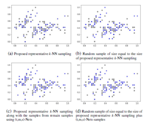
Figure 5: Training sample selection (i.e., represented by blue star scatter-plot point) from IRIS dataset with four different strategies.

The Figure 8 shows the four different 2D scatter-plot representation of MNIST dataset. In Figure 8(a), we are representing the 2D scatter-plot of sampled t-SNE along with the interpolation of inliers and placement of outliers. The sampled t-SNE is designed based on the best representative sample of the representative k-NN sampling-based clustering concerning the best clustering technique. The inliers of remaining samples (i.e, other than representative samples) are interpolated to t-SNE with the parameter r_x that is obtained from the proposed heuristic. The outlier of remaining samples are placed into an existing t-SNE environment based on the Boystov et.al heuristic.

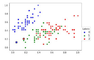
Figure 6: The 2D scatter-plot of IRIS data which denotes the outliers from the newly added sample with proposed heuristic.

In Figure 8(a), the outliers are placed separately from other embedding points. The Figure 8(b) shows the 2D scatter-plot of (t,m,s)-Nets based t-SNE along with interpolation of other samples. The (t,m,s)-Nets based t-SNE is designed with a combination of representative k-NN sampling-based clustering and (t,m,s)-Nets of remaining samples. The (t,m,s)-Nets samples are selected from the data samples, which are having NN-score as zero after selecting the samples using a mutual k-NN sampling with a static graph updation algorithm. The inliers of remaining samples (i.e, other than representative samples plus (t,m,s)-Nets samples) are interpolated to t-SNE with the parameter r_x that is obtained from the Boystov et.al heuristic. The Figure 8(c) and 8(d) shows the 2D scatter-plots of a random sampled t-SNE along with the addition of new data samples. The random sample size is equal to the sample size of Figure 8(a) and 8(b). The inliers and outliers of remaining samples are placed according to the intuitions of Figure 8(a) and 8(b). The representative k-NN sampling-based results are statistically significant than the random sampling based results which is derived in our earlier paper [19]. The following section describe the conclusion and future work.

6. Conclusion and Future Work

In this paper, we have proposed a representative k-NN samplingbased clustering approach, which generates cluster results on a sampling basis. The most frequently used clustering techniques are applied to obtain the sampling-based cluster results. Initially, we determine the applicable set of techniques for the given dataset. From the applicable set, sampling-based clustering results of each technique are evaluated by an external cluster validation index called FMI-score. The applicable techniques are arranged in an orderly sequence of their FMI scores. Some threshold parameter derives the recommendation of clustering techniques for the given dataset. From the recommended set, the first technique is selected as the most desirable clustering for the given dataset.

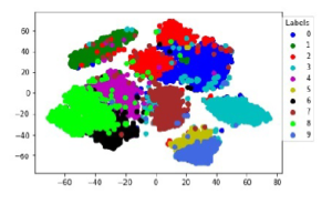
Figure 7: The baseline 2D visual representation of Representative k-NN samplingbased clustering t-SNE embedding where t-SNE applied on whole data

The samples of this technique are used for generating the lowdimensional embedding of input data. The embedding results are visualized and quantitatively evaluated in the context of samplingbased cluster results. The proposed approach is expanded to identify all the applicable set of clustering techniques for the given dataset, which can be done as future work. There is scope for implementing the proposed algorithm in a distributed environment that can be applied to Big Data.

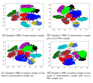
Figure 8: 2D representation of four different t-SNE embedding of MNIST dataset, (a) t-SNE embedding of representative train sample and the interpolation of inliers as well as placement of outliers with proposed heuristic, (b) t-SNE embedding of representative train sample which includes the samples from (t,m,s)-Nets and the interpolation of inliers as well as placement of outliers with A Boystov et.al heuristic, (c) t-SNE embedding of random sample of size equal to the size of sub-figure (a) and the interpolation of inliers as well as placement of outliers with proposed heuristic, (d) t-SNE embedding of random sample of size equal to the size of sub-figure (b) and the interpolation of inliers as well as placement of outliers with A Boystov et.al heuristic.

Acknowledgment

I would like to express my sincere gratitude to Visveswaraya PhD Scheme for providing financial support to pursue my PHD degree.

1. Matthew Partridge, Rafael A Calvo, ”Fast dimensionality reduction and simple PCA” Intelligent data analysis, 2(3), 203–214, 1998.
2. Trevor F Cox, Michael AA Cox, Multidimensional scaling, Chapman and hall/CRC, 2000.
3. Jianbo Shi, J. Malik, ”Normalized cuts and image segmentation” IEEE Trans- actions on Pattern Analysis and Machine Intelligence, 22(8), 888–905, 2000, doi: 10.1109/34.868688.
4. Joshua B Tenenbaum, Vin De Silva, John C Langford, ”A global geomet- ric framework for nonlinear dimensionality reduction” Science, 290(5500), 2319–2323, 2000. DOI: 10.1126/science.290.5500.2319
5. Sam T Roweis, Lawrence K Saul, ”Nonlinear dimensionality reduction by locally linear embedding” Science, 290(5500), 2323–2326, 2000. DOI: 10.1126/science.290.5500.2323
6. Mikhail Belkin, Partha Niyogi, ”Laplacian eigenmaps for dimensionality re- duction and data representation” Neural computation, 15(6), 1373–1396, 2003. https://doi.org/10.1162/089976603321780317
7. Geoffrey E Hinton, Sam T Roweis, ”Stochastic neighbor embedding” in Ad- vances in neural information processing systems, pages 857–864, 2003.
8. Laurens Van Der Maaten, Eric Postma, Jaap Van den Herik, ”Dimensionality reduction: a comparative” J Mach Learn Res, 10(66–71),13, 2009.
9. Laurens Van Der Maaten, Geoffrey Hinton, ”Visualizing data using t-sne” J Mach Learn Res, 9(Nov):2579–2605, 2008.
10. Wentian Li, Jane E Cerise, Yaning Yang, Henry Han, ”Application of t-sne to human genetic data” Journal of Bioinformatics and Computational Biology, 15(4):1750017, 2017. https://doi.org/10.1142/S0219720017500172
11. Minh Nguyen, Sanjay Purushotham, Hien To, Cyrus Shahabi, ”m-tsne: A framework for visualizing high-dimensional multivariate time series” arXiv preprint arXiv:1708.07942, 2017.arXiv:1708.07942
12. Walid M Abdelmoula, Benjamin Balluff, Sonja Englert, Jouke Dijkstra, Marcel JT Reinders, Axel Walch, Liam A McDonnell, Boudewijn PF Lelieveldt, ”Data-driven identification of prognostic tumor subpopulations using spatially mapped t-sne of mass spectrometry imaging data” in Pro- ceedings of the National Academy of Sciences, 113(43):12244–12249, 2016. https://doi.org/10.1073/pnas.1510227113
13. Laurens Van Der Maaten, ”Accelerating t-sne using tree-based algorithms” J Mach Learn Res, 15:3221–3245, 2014.
14. Nicola Pezzotti, Boudewijn PF Lelieveldt, Laurens Van Der Maaten, Thomas Ho¨llt, Elmar Eisemann, Anna Vilanova, ”Approximated and user steerable tsne for progressive visual analytics” IEEE transactions on visualization and com- puter graphics, 23(7):1739–1752, 2016. DOI: 10.1109/TVCG.2016.2570755
15. Laurens Van Der Maaten, ”Learning a parametric embedding by preserving local structure” in Artificial Intelligence and Statistics, pages 384–391, 2009.
16. Andrej Gisbrecht, Alexander Schulz, Barbara Hammer, ”Parametric nonlinear dimensionality reduction using kernel t-sne” Neurocomputing, 147:71–82, 2015. https://doi.org/10.1016/j.neucom.2013.11.045
17. Andrey Boytsov, Francois Fouquet, Thomas Hartmann, Yves LeTraon, ”Visu- alizing and exploring dynamic high-dimensional datasets with lion-tsne” arXiv preprint arXiv:1708.04983, 2017. arXiv:1708.04983
18. Stephen Ingram, Tamara Munzner, ”Dimensionality reduction for docu- ments with nearest neighbor queries” Neurocomputing, 150:557–569, 2015. https://doi.org/10.1016/j.neucom.2014.07.073
19. Bheekya Dharamsotu, K. Swarupa Rani, Salman Abdul Moiz, C. Raghaven- dra Rao, ”k-NN sampling for visualization of dynamic data using LOIN- tSNE” in 2019 IEEE 26th International Conference on High Perfor- mance Computing, Data, and Analytics (HiPC), pages 63–72, 2019. DOI: 10.1109/HiPC.2019.00019
20. L. J. Williams, H. Abdi, “Fishers least significant difference (lsd) test,” Ency- clopedia of research design, 218, 840–853, 2010.
21. Tapas Kanungo, David M Mount, Nathan S Netanyahu, Christine D Piatko, Ruth Silverman, Angela Y Wu, ”An efficient k-means clustering algorithm: Analysis and implementation” IEEE Transactions on Pattern Analysis and Ma- chine Intelligence, 24(7):881–892, 2002. DOI: 10.1109/TPAMI.2002.1017616
22. Wei Zhang, Deli Zhao, Xiaogang Wang, ”Agglomerative clustering via maxi- mum incremental path integral” Pattern Recognition, 46(11):3056–3065, 2013. https://doi.org/10.1016/j.patcog.2013.04.013
23. Tian Zhang, Raghu Ramakrishnan, Miron Livny, ”BIRCH: an efficient data clustering method for very large databases” ACM Sigmod Record, 25(2):103– 114, 1996. https://doi.org/10.1145/235968.233324
24. James C. Bezdek, Robert Ehrlich, William Full, ”FCM: The fuzzy c-means clustering algorithm” Computers and Geosciences, 10(2):191–203, 1984.
25. Erich Schubert, Jo¨ rg Sander, Martin Ester, Hans Peter Kriegel, Xiaowei Xu, ”DBSCAN revisited, revisited: why and how you should (still) use DB- SCAN” ACM Transactions on Database Systems (TODS), 42(3):1–21, 2017. https://doi.org/10.1145/3068335
26. John Carlo Dassun, Argie Reyes, Hideo Yokoyama, P Bibangco El Jireh, Mehreen Dolendo, ”Ordering points to identify the clustering structure algo- rithm in fingerprint-based age classification” Virtutis Incunabula, 2(1):17–27, 2015.
27. Dorin Comaniciu, Peter Meer, ”Mean shift: A robust approach toward feature space analysis” IEEE Transactions on Pattern Analysis and Machine Intelli- gence, 24(5):603–619, 2002. DOI: 10.1109/34.1000236
28. Ulrike Von Luxburg, ”A tutorial on spectral clustering” Statistics and Comput- ing, 17(4):395–416, 2007.
29. Douglas A Reynolds, ”Gaussian mixture models” Encyclopedia of biometrics, 741, 2009.
30. Brendan J. Frey, Delbert Dueck, ”Clustering by passing messages between data points” Science, 315(5814):972–976, 2007. DOI: 10.1126/science.1136800
31. David Sculley, ”Web-scale k-means clustering” in Proceedings of the 19th international conference on World Wide Web, pages 1177–1178, 2010. https://doi.org/10.1145/1772690.1772862
32. Edward B Fowlkes, Colin L Mallows, ”A method for comparing two hierarchi- cal clusterings” Journal of the American Statistical Association, 78(383):553– 569, 1983.
33. Y. Liu, Z. Li, H. Xiong, X. Gao, J. Wu, S. Wu, ”Understanding and en- hancement of internal clustering validation measures” IEEE Transactions on Cybernetics, 43(3):982–994, 2013. DOI: 10.1109/TSMCB.2012.2220543
34. Shusaku Tsumoto, ”Contingency matrix theory: Statistical dependence in a contingency table” Information Sciences, 179(11):1615–1627, 2009. https://doi.org/10.1016/j.ins.2008.11.023
35. Amit Saxena, Mukesh Prasad, Akshansh Gupta, Neha Bharill, Om Prakash Patel, Aruna Tiwari, Meng Joo Er, Weiping Ding, Chin-Teng Lin, ”A review of clustering techniques and developments” Neurocomputing, 267:664–681, 2017. https://doi.org/10.1016/j.neucom.2017.06.053
36. Anil K Jain, M Narasimha Murty, Patrick J Flynn, ”Data cluster- ing: a review” ACM computing surveys (CSUR), 31(3):264–323, 1999. https://doi.org/10.1145/331499.331504
37. Pavel Berkhin, ”A survey of clustering data mining techniques” in Grouping multidimensional data, pages 25–71. Springer, 2006.
38. Andrew Y Ng, Michael I Jordan, Yair Weiss, ”On spectral clustering: Analysis and an algorithm” in Advances in neural information processing systems, pages 849–856, 2002.
39. George C Linderman, Stefan Steinerberger, ”Clustering with t-sne, prov- ably” SIAM Journal on Mathematics of Data Science, 1(2):313–332, 2019. https://doi.org/10.1137/18M1216134
40. Donald Shepard, ”A two-dimensional interpolation function for irregularly- spaced data” in Proceedings of the 1968 23rd ACM national conference, pages 517–524, 1968. https://doi.org/10.1145/800186.810616
41. Jarkko Venna, Samuel Kaski, ”Neighborhood preservation in nonlinear projec- tion methods: An experimental study” in International Conference on Artificial Neural Networks, pages 485–491. Springer, 2001.
42. T. Kollig, A. Keller, ”Efficient multidimensional sampling” Computer Graphics Forum, 21(3), 2002.
43. Dheeru Dua, Casey Graff, UCI machine learning repository, 2019.
44. Bernhard Scho¨lkopf, Alexander Smola, Klaus-Robert Mu¨ller, ”Kernel principal component analysis” in International conference on artificial neural networks,
    pages 583–588. Springer, 1997.

(Click Here)

(Click Here)