1. Introduction

Currently, the manufacturers have equipped with standard safety systems in researching the production of autonomous vehicles. However, in the context of traffic in complex environments, with the development of technology, the safety standards for autonomous vehicles have been raised, in which the driver assistance technology is a problem that needs to be cared about creating safe movements for vehicle. This technology can be mentioned by tracking driving conditions such as road conditions, vehicle status information, sensor technology, etc. to contribute to the development of advanced driver-assistance technology. For example, technology that supports the safety system in the adaptive cruise control system helps maintain distance from the vehicle ahead, collision avoidance assistance system helps predict collisions with obstacles with timely braking, as well as the lane keeping system helps the vehicle recognize the separator to adjust the vehicle direction so that the vehicle is always moving in the middle of the lane.

However, the scenario that these systems handle may be relatively simple compared to the diverse and complex situations we often encounter in traffic environment conditions. To solve this problem, we offer a motion control assistance solution to create a safe motion trajectory for the vehicle. The design of this control support system has two main goals: the first is minimal intervention – that is, applying autonomous control only when necessary, the second is to ensure safety – meaning the vehicle’s collision-free state is clearly enforced through optimal constraints.

 The control support solution we propose in this article is implemented by predictive control based on the non-linear model predictive control and optimize the steering support system by the steering system along with the acceleration of the vehicle. In the solution assuming the current position of the vehicle, road boundaries, vehicles ahead and uncertain predictions about the future state of the vehicle in the form of a parametrized posterior distribution by their mean and covariance are known. Specifically, for this solution, we will combine the uncertainty changes over time to the mobile obstacle predictions into the optimization problem, and also introduce constraints for boundary limits and moving obstacles while maintaining a vehicle’s movement plan for a limited time.

The next section of the paper will introduce the basic principles of predictive control and thereby propose a control solution based on Non-linear Model Predictive Control. Next is the experimental section and conclusion with some suggestions for further research directions for the problem of autonomous vehicles.

2. Building solution to support motion control

Theoretically, in order for an autonomous vehicle to avoid collisions, we need to calculate to find the set of states in which the vehicle may encounter a collision situation when participating in traffic and then control the movement so that the vehicle does not move into that state set. There are many studies [1]-[5] doing this task that have determined the inevitable collision state set or target motion set. However, these studies do not limit the applicability or make assumptions for simple traffic scenarios, so it is difficult to analyze calculations. In this paper, the solution that we propose is the idea of defining collision state set and thereby determining the set of probability constraints to avoid collisions. At the same time, in this solution, we combine the steering speed control and increase/decrease speed so that the collision avoidance effect can be realized better. The ideas have originated from the studies [6,7,8,9] in the process of determining the difference of the steering angle or the deviation of the front wheel to achieve a safe trajectory.

In many studies, the model predictive control (MPC) has been applied to control autonomous vehicle [7]-[11] as the MPC approach to plan motion based on the vehicle’s basic movements and track the road to avoid obstacles, or the MPC approach without constraint conditions and determine the stability of the vehicle with the surrounding environment to provide a safe steering angle at constant speed in a discrete environment. In this article, the MPC approach that we use can handle complex situations with steering control, increase/decrease vehicle speed, and avoid mobile obstacles at a certain extent in an uncertain environment.

The cost function of most MPC methods [7], [11]-[13] often depends on the time and the constraints on the path, so it needs to be pre-optimal or specific time steps or generated out and track the fixed motion of the vehicle, this leads to differences in result from the initial conditions of optimization that could result in invalid linear constraints and unpredictable motion planning. Therefore, we apply the point processing method in [14] and directly solve the nonlinear model predictive control problem by focusing on providing all costs and constraints for the decoding set that does not need to be linear manually.

2.1.  Statement of problems

This problem is built on two basic principles: the first is minimal intervention, the second is to ensure safety, meaning the probability of a collision involving the surrounding environment and other traffic objects must be below certain thresholds. And this problem is done in discrete time intervals , with  (  is the current time,  is the i time step of the plan).

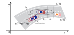
Figure 1. Modeling of autonomous vehicle and other vehicles

At interval k, with values of position , linear velocity , direction of vehicle  and steering angle , the mathematical model of the vehicle is determined by the set .

Assuming   is the occupied area of the vehicle at  state (illustrated in Figure 1, with autonomous vehicle modeled by linked circles), the input values on the control using  steering speed and  acceleration is assigned by .

Thus, the future state of the vehicle is represented by a discrete dynamic system as follows:

With other objects in traffic such as different kinds of car, bicycles, pedestrians, etc. called other objects will be assigned by the index , the input control and their configuration parameters are determined by the values ​​of  and .

In order to combine uncertainty, it is necessary to assume that the future state distributions of the objects at  future time intervals is known. They are parameterized to the average state value   and covariance . Therefore, the degree of uncertainty in the forecast can be reflected through the covariance value  .

At each given state, each object will occupy one space  having probability greater than  (  is the acceptable probability of collision that may happen), the model of the object and this occupied space are shown in Figure 1.

The free space defined in this problem is the workspace  and the location map of obstacles  containing static obstacles such as limit of roads and systems of seperator, etc., at the same time, the surrounding environment is determined to be the state of other objects (including means of traffic, obstacles) at the time .

In this study, with the set of states  and input set , we will build a general discrete time constraint optimization at  time steps with a time limit .

Thus, the goal of the solution is to calculate the optimal input values ​​  for autonomous vehicle with minimizing cost function .

In which:  is the minimum cost to minimize deviations from the input value , and  is the cost depending on the properties of the trajectory according to the motion plan.

This optimum problem follows a set of constraints: the first is to use the vehicle transition model, the second is the non-collision constraint with static obstacles and the third is the probability that no collision will occur  with other traffic participants.

And the optimal trajectory of the vehicle is given as follows:

 ,  with : are parameters for all other traffic objects,  is the initial state of vehicle.

2.2.   Building a solution

The solution was built to calculate the creation of a safe motion trajectory with a predefined horizon. Optimal problems are constrained by cost values, transition models, maintaining vehicle movement within the boundaries of the lane median, and avoiding collisions with other road participants that must ensure the probability of collision below the value .

In solutions using model predictive control of previous studies [7,11,13], the researchers often use factors such as constant longitudinal speed and small angle assumptions in scenarios avoiding obstacles on the straight road. In this study, we will consider the impact of longitudinal speed to ensure overall safety in complex traffic environments.

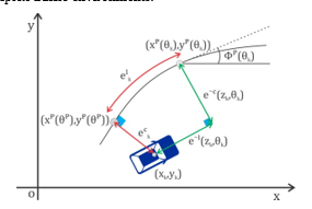
Figure 2. Vehicle dynamics model

The vehicle model in this solution has been introduced with a fixed rear wheel and the motion control is located on the front wheel with  and  states set here, and the control of rear wheel movement is via center bridge with distance  and a continuous dynamic model. This motion model is described by a discrete time model with integrals , as follows:

In this model, the limits applied include steering angle , steering speed  and longitudinal speed . The introduction of these limits is consistent with vehicle performance and road traffic rules, as well as a number of restrictions will be set to ensure safety such as speed limits when moving into the corners by limiting the slip coefficient  and limiting the maximum speed quickly by the acceleration limit .

The model predictive control method in this study is based on model predictive contouring control method [15,16,17] and is used to solve problems, in this study, it is not required that the motion trajectory of the vehicle must be exactly according to the reference trajectory, but the motion trajectory must be in the safe range.

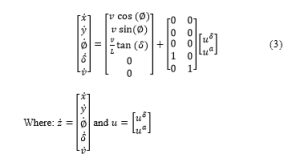
On the reference trajectory, the process takes place as follows:

At time , the vehicle is in position , the process of following the reference path is limited and continuously differentiable in geometric space  of path parameter , with the tangential vector  and the normal vector  as follows:

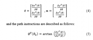
the path parameterized according to the arc length  will allow to estimate the vehicle’s progress with  on the reference path and the actual path  if during the parameterization of the curves the arc length is negligible and the distance between the points is small compared to the arc length. At the same time, since the motion trajectory of the vehicle will follow a certain path and have a slight deviation from the reference trajectory determined by the road boundary, we can assume that the trajectory remains the same offset, so: , with this additional assumption will generate an approximate process according to the path parameter, as follows:

where  describes the approximation process in time step .

In the general case, finding the path parameter  of the nearest point  on the reference path is not feasible and not suitable for fast optimization. Therefore, the value of  will be approximated according to equation (6).

During the motion planning process, if the actual path deviates from the reference path, the delay error from the first approximation point in time progression to the next point and the position error referenced to the horizontal roads  along the tangential path  are defined as follows:

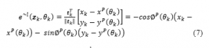
If the delay error  is small, the process of constructing an approximate path will be as close to the horizontal asymptote as  and . Also, in the process of optimizing the prediction control, the delay error should be actively handled so that the error of the predictive process  is small enough according to the motion planning process.

When projected on the standard path between the actual position and the predicted position, we will determine the contouring error by the deviation of these two positions, as follows:

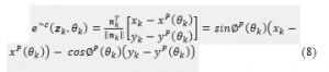
and the contouring error is a standard for establishing good motion planning when the vehicle is in motion not deviated from a given reference path. Therefore, the cost function of predictive state control is built based on the balance between the contouring error factors , delay error  and the process of building approximate path  to achieve the best combination, as follows:

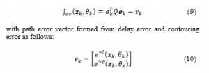
For the performance of the path, all reference paths are parameterized by  – a continuous clothoid path in a system of paths through predetermined points. The clothoid path estimate will be replaced by the third-order spline function of equally spaced nodes and parameterization of the spline functions along the arc length is sufficiently accurate, as well as achieves good performance in the calculation. Because the spline functions provide an analytical parameter about the reference path, the limit of the path and the derivatives needed to solve the nonlinear optimization problem.

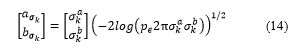
At position , from the projection along the normal of the reference path at the actual culvilinear abscissa , we get the lateral distance with the reference path and approx slag equal to such that . Just as the movable space of autonomous vehicles at the crossroads  is limited by the left boundary , the right boundary   of the lane and other static obstacles will be parameterized by the third order spline function to allow analytical evaluation and derivation.

As such, the horizontal traverse for the path is limited as follows:

where:  is the upper limit of the vehicle position projection on the standard reference path and this value is greater than  of the vehicle width. At the same time, maintaining the validity of  as a limit just taking the radius of the vehicle’s operating range as an upper limit is enough to ensure safety.

Because the relationship between the path and the direction of the vehicle is relative, we need to establish a constraint between the direction of the path  and the movemen direction of the vehicle , as follows:

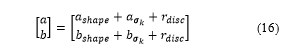
In the solution of this study, other traffic participants will be described by an orientation ellipse  with  being a semi-major axis and  being a semi-minor axis of the ellipse in the longitudinal and horizontal directions of the objects.

The development of future trajectories of these objects is assumed to have some uncertain positions of posterior distribution and is parameterized by the average trajectory  and degree uncertainty , as follows:

In the general case, we propose a model for generating indeterminate positions of vehicles with uncertainty  at the time  and  is the uncertainty incurred. Therefore, the value of the variance is determined to approximate to adjust the direction of the vehicle motion aligning the main axis of the surrounding ellipse. The generation of indeterminate positions in the horizontal direction of the vehicle is limited by a maximum value to consider the maximum rationality of the maximum flow of vehicles currently in the current lanes.

The level-set of Gaussian  describe the indefinite position of other road users at  degree and ellipses formed with coefficients are set as follows:

Therefore, we can use the main axis direction and add coefficients to the cross axles of the vehicle to identify the area of ​​the obstacle with the probability of occupancy above the threshold . At the same time, the rectangular area used to determine the position and occupied area of ​​autonomous vehicles will be replaced by a set of circulars with radius . The use of circles instead of ellipses represents obstacles because the presence of an autonomous vehicle does not need to be aligned in a straight axis, and Minkowski’s sum calculation efficiency is not possible if shown by ellipses whose axes do not fit tightly. The Minkowski sum of the sets of circles surrounding the vehicle and the collision constraints shown by the previous displaced ellipses are calculated as follows:

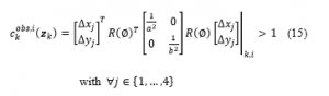
where ,  are the distances from the circle set covering the area around the vehicle to the center of obstacle  at the time  and  is the rotation matrix corresponding to the motion direction of the obstacle, and the semi-major axis of the constraint ellipse. The result is calculated as follows:

Thus, we have a collision-free constraint with a higher probability  than other means.

As our goal of the solution in this research is to minimize the intervention of the driving, that is, the control system only intervenes with the steering operation when really necessary with the minimum intervention time:

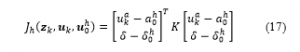
where  is the inconsistent value of system state,  is the steering angle value and  is the acceleration value at the time .

In the process of setting values for control inputs, we only determine the steering angle value  and acceleration  without determining the steering speed value . However, in the general case if the front view angle can be controlled, the speed value is still used as the input value, and the control process  maintains the steering speed and acceleration of the vehicle.

The calculation of the trajectory cost will include the cost of the model predictive control calculated by the equation , and at the same time add input control deviations and slip coefficients to create smooth and comfortable trajectories when the vehicle is in motion. The weights  and  allow for sorting based on different priorities, so the trajectory cost is calculated as follows:

where  has transformed the inconsistency from the reference path error into a better direction of motion.

Finally, the solution proposed is the optimization problem. It is done by the minimum factor combining linear between the cost of intervention into the system and trajectory cost, as follows:

in which, the weight  and exponential decay function  are used to enhance the input value for the system.

We have chosen the solution to make the weight  reach a high value, so that when moving forward in the predictive model, the system will be able to respond well to inputs but still depend on . By doing so, the solution presented in this study can plan a full implementation without having to predict the planned motion trajectory. Therefore, the nonlinear optimization problem with constraints on state, dynamics, paths and obstacles is constructed as follows:

with initial initialization values for the path , the left boundary  and the right boundary  set by the arc and the static obstacles that the vehicle is moving. At the same time, in each loop when the system executes the initial states  and , the input variables  and predicts other objects of traffic   will be given a predictive model for the control system. After that, the optimal solution given by equation (20) and the optimal control will be executed by the system.

3. Experimental results

To test and evaluate the proposed solution, we have conducted empirical simulation of processes in the matlap environment. At the same time, in order to ensure the objectivity and reliability when evaluating, we have conducted simulations with different scenarios and autonomous vehicles controlled moving with steering angle  and desired acceleration . Input variables will be handled using model predictive control to ensure generating safe movement, the reference path and the left boundary , right boundary  are designed and determined accordingly with the road system. During the experiment, the calculations uses SI measurement system with sampling interval of 0.1s, the trajectory is transferred to I/O controller with simulation time of 0.005s.

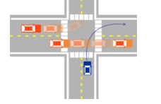
Figure 3. Simulating the scenario 1

Scenario 1: In this scenario, the autonomous vehicle will move into a corner, with the input values ​​for the control system will be able to make the vehicle’s direction of travel out of the limit of traffic lanes. At this point, the driver assistance system will perform braking to reduce the vehicle speed to the safe speed limit with the coefficient constraint before the car enters a corner, then increase the vehicle speed after going out of the corner to ensure the progress in the motion planning. With such a driver assistance process, it shows the advantages of controlling the longitudinal force, horizontal force and acceleration the vehicle, as well as implementing the vehicle’s movement plan that is complete when entering corners with the brake and increase/decrease speed operations.

Scenario 2: In this scenario, the autonomous vehicle will implement the movement plan from the slip road and turn left to enter the main traffic lane, the initial positions and the speed of other traffic participants  are initialized randomly. To increase the time span of the planning without adjusting the calculations, we will take the approach of changing the distance at each step as follows: The first 40 steps have a distance of   and the next 50 steps have , which leads to a planning time of 24 seconds for all calculations to be performed in real time.

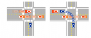
Figure 4. Simulating the scenario 2

The process of following this scenario will be repeated many times with randomly generated input values ​​and there are times when the input values ​​are insecure input to the system, which will lead to accident when the vehicle is moving as planned. However, with the control support system that our solution offers, it is possible to prevent incidents in the most likely cases of accidents.

Specifically: The planning process of movement when the vehicle is moving in a slip road before entering the main road, a collision may occur with the right boundary of the lane. After that, to move into the main lane, the vehicle turns left, at this time on the main lane, other vehicles are moving complicatedly, and unsafe situations may occur. To handle this movement of the vehicle, the control support system will activate the brakes to bring the vehicle’s motion status to a stop state so that other vehicles in traffic can move through it, until the safe distance between the autonomous vehicle and other vehicles is large enough, the system activates the vehicle velocity so that the vehicle can move over the cross and merge into the main lane.

During the experiment, we can see that the uncertainty in the predictive of other vehicles is very important because the future states of the predictive model can deviate from the desired predictive point. In the case of omitting uncertainty, the motion planning process needs to provide more precise and specific constraints to ensure the vehicle safety.

4. Conclusions

This paper has proposed a motion control assistance solution to ensure the safety of an autonomous vehicle. The optimal feature of this solution is to shorten the motion planning cycle to minimize deviations from inputs of the prediction while ensuring movement safety. This controller support solution is only implemented in situations where a complex vehicle movement scenario is likely to have a collision with realistic warning elements.

The main idea of ​​this technical solution will support designing an autonomous vehicle with a safe stop whatever the current vehicle control. The experimental simulation with the given scenarios shows that the safety factor can be achieved by calculating to consider all possible possibilities of other vehicles.

In the future, in order that this solution will be more reliable, we have experimented the settings by transferring the simulation to the real environment with experimental vehicle equipped with sensors. When experimenting on reality, it will add a number of factors to analyze the stability of the system so that the behavior of traffic participants is more accurately forecasted. The extensive implementation of this driver-assistance solution for semi-autonomous or autonomous vehicles in vehicle control systems will be able to minimize the amount of damage and create a safe movement plan for the future.

1. A. Bautin, L. Martinez-Gomez, T. Fraichard, “Inevitable Collision States: A probabilistic perspective,” IEEE International Conference on Robotics and Automation 2010,pp.4022–4027,2010,DOI: 10.1109/ROBOT.2010.5509233.
2. D. Althoff, M. Althoff, D. Wollherr et al, “Probabilistic collision state checker for crowded environments,” IEEE International Conference on Robotics and Automation – 2010, pp. 1492–1498, 2010, DOI: 10.1109/ROBOT.2010.5509369.
3. D. Hoehener, G. Huang, D. D. Vecchio, “Design of a lane departure driver-assist system under safety specifications,” IEEE 55th Conference on Decision and Control (CDC)-2016, pp. 2468–2474, 2016, DOI: 10.1109/CDC.2016.7798632.
4. M. Forghani, J. M. McNew, D. Hoehener et al, “Design of driver-assist systems under probabilistic safety specifications near stop signs,” IEEE Transactions on Automation Science and Engineering, vol. 13, no. 1, pp. 43–53, 2016, DOI: 10.1109/TASE.2015.2499221.
5. T. Fraichard, H. Asama, “Inevitable collision states. A step towards safer robots?” Advanced Robotics, vol. 18, no. 10, pp. 1001–1024, 2003, DOI: 10.1109/IROS.2003.1250659.
6. J. Alonso-Mora, P. Gohl, S. Watson et al, “Shared control of autonomous vehicles based on velocity space optimization,”IEEE International Conference on Robotics and Automation (ICRA)-2014, pp. 1639–1645, 2014, DOI: 10.1109/ICRA.2014.6907071.
7.  S. Erlien, S. Fujita, J. C. Gerdes, “Shared steering control using safe envelopes for obstacle avoidance and vehicle stability,” IEEE Transactions on Intelligent Transportation Systems, vol. 17, no. 2, pp. 441–451, 2015, DOI: 10.1109/TITS.2015.2453404.
8. V. A. Shia, Y. Gao, R. Vasudevan et al, “Semiautonomous vehicular control using driver modeling,” IEEE Transactions on Intelligent Transportation Systems,vol.15,no.6,pp.2696–2709,2014, DOI: 10.1109/TITS.2014.2325776.
9.  Y. Gao, A. Gray, A. Carvalho et al, “Robust nonlinear predictive control for semiautonomous ground vehicles,” in 2014 American Control Conference, pp. 4913–4918, 2014, DOI: 10.1109/ACC.2014.6859253.
10. A. Gray, Y. Gao, T. Lin et al, “Predictive control for agile semi-autonomous ground vehicles using motion primitives,” American Control Conference (ACC)-2012, pp. 4239–4244, 2012, DOI: 10.1109/ACC.2012.6315303.
11. S. J. Anderson, S. B. Karumanchi, K. Iagnemma, “Constraint based planning and control for safe, semi-autonomous operation of vehicles,” IEEE Intelligent Vehicles Symposium-2012, pp. 383–388, 2012, DOI: 10.1109/IVS.2012.6232153.
12. B. Paden, S. Z.Yong, D. Yershov et al, “A survey of motion planning and control techniques for self-driving urban vehicles,” IEEE Transactions on Intelligent Vehicles, vol. 1, no. 1, pp. 33–55, 2016, DOI: 10.1109/TIV.2016.2578706.
13. S. J. Anderson, S. C. Peters, T. E. Pilutti et al, “An optimal-control-based framework for trajectory planning, threat assessment, and semi-autonomous control of passenger vehicles in hazard avoidance scenarios,” International Journal of Vehicle Autonomous Systems, vol. 8, no. 2-4, pp. 190–216, 2010, DOI: 10.1504/IJVAS.2010.035796.
14. A. Domahidi, J. Jerez ,“FORCES Pro,” embotech GmbH (http://embotech.com/FORCES-Pro), 2014.
15. A. Liniger, A. Domahidi, M. Morari, “Optimization-based autonomous racing of 1:43 scale RC cars ,” Optimal Control Applications and Methods, vol. 36, no. 5, pp. 628–647, 2017, DOI: 10.1002/oca.2123.
16. D. Lam, C. Manzie, M. C. Good, “Model predictive contouring control for biaxial systems,” IEEE Transactions on Control Systems Technology, vol. 21, no. 2, pp. 552–559, 2013, DOI: 10.1109/TCST.2012.2186299.
17. T. Faulwasser, B. Kern, R. Findeisen, “Model predictive pathfollowing for constrained nonlinear systems,” in Proceedings of the 48th IEEE Conference on Decision and Control (CDC) held jointly with 2009 28th Chinese Control Conference, pp. 8642–8647, 2009, DOI: 10.1109/CDC.2009.5399744.

(Click Here)

(Click Here)