1. Introduction

This paper is an extension of work originally presented in The 11th IEEE International Conference on Knowledge and Systems Engineering (KSE) 2019 in Da Nang, Vietnam [1].

Recent years, the field of health care has been receiving great attention from the world. Many services and high-tech applied equipment are manufactured for medical use. Medical results require high accuracy and meet a wide range of diseases, so it is necessary to deploy diagnostic methods and treatments with new technologies. Also, dangerous diseases such as Liver Cirrhosis, Colorectal, HIV, etc. have an increasing rate due to lifestyle, way of life, diet. Liver Cirrhosis is a disease of concern due to the increasing trend each year. The main cause of cirrhosis is the living environment, using a lot of alcohol, toxic chemicals. The level and duration of consumption is an important determinant of the deaths 2,494 compared to 2014 [2]. Colorectal cancer is the third most common disease in the United States. The main object of the disease is elderly but the proportion of young people with the disease tends to increase. According to statistics in early 2020, an estimated 53,200 deaths (28,630 males and 24,570 females) are due to the disease, but there is an increased incidence in young people. Although the incidence decreases by 3.6% per year from 2007 to 2016 in adults 55 years and older, they increase 2% per year in adults under 55 years. This year, colorectal cancer is estimated to be the fourth most commonly diagnosed cancer in the United States for men and women aged 30 to 39 [3]. Heart failure is a common complication of Cardiometabolic diseases (CMD). When the pumping action of the heart weakens, the amount of blood pumped out is insufficient for the body to make it difficult for the person to feel short of breath, or chest pain, which is called heart failure. Genetic diversity has not been considered in the diagnosis and prognosis of the disease. We apply a single method of treatment to all patients with a similar diagnosis. The results showed that some patients’ health did not improve, and the rest gradually recovered. This shows that many methods need to be applied for an effective treatment for each patient. Advances in data processing technology make us understand the importance of metagenomic to human health and explore the diversity of genetics. Deep learning has provided many algorithms to help scientists propose models, methods of diagnosis and treatment.

Modern techniques in healthcare are still developing at a great speed. One of them is Personalized Medicine which defines the impact goals that will work for a patient based on the patient’s environmental factors, genes, etc. and is used on a group of patients. Today, scientists have studied numerous methods for Personalized Medicine and metagenomic is one of them. As we have known, metagenomics is a method of sequencing and analyzing the DNA of microorganisms collected from the environment without culturing them. We are looking at the human gut environment. Bacteria are often very diverse, they are classified into seven basic types: domain, kingdom, phylum, class, order, family, genus, and species. This diversity helps to provide more information about diseases to support more effective diagnosis and prognosis. The diseases under consideration are complex and we only have a limited number of observation data samples, so the prediction tasks are produced in inconsistent results with comparable diseases.

To test and propose models for healthcare services, Machine learning algorithms have been strongly researched and developed to solve metagenomics-related problems , mainly prediction genes [4,5], Operational Taxonomic Unit clustering [6–9], comparative metagenomics [10–13], binning, taxonomic profiling and assignment [14]. All of the issues mentioned are given in [14].

The authors presented the basic principles of machine learning in [15] and a typical pipeline was introduced [16,17]. This model is clustered or classified based on pre-processed results and feature extraction. A machine learning program consists of three basic components, such as data (or experience), task (formed by the output of the algorithm) and target (possibly in the form of measuring the efficiency of the output). MetAML was introduced in [17] by Edoardo et al. which is a computational framework that learns about the presence of specific species signs and the relative abundance of species, these two collectively called are quantitative microbiome configurations. Using machine learning to independently evaluate the accuracy of models on large metagenomic datasets, thereby analyzing and comparing the practical microbiome usage strategies that were recommended in [18]. With the task of classifying metagenomics, Ph-CNN [19] was introduced to the OTU hierarchical structure and it was also compared to other technologies in machine learning such as random forests. PopPhy-CNN [20] is introduced by D. Reiman et al. PopPhy-CNN is deep learning framework, using embedded information based on a phylogenetic tree to predict diseases from metagenomic data. PopPhy-CNN has superior performance compared to random forests, support vector machines, LASSO and the basic 1D-CNN model built with bacterial vectors. In addition to retrieving information microbiological classifications from trained CNN models, PopPhy-CNN also visualizes phylogenetic tree classifications. Several deep learning algorithms have been evaluated as a feasible approach to speed up DNA sequencing [21]. To identify viruses by deep learning with metagenomic data, J. Ren et al. [22] proposed using DeepVir Downloader (a reference-free and alignment-free machine learning method) to improve accuracy and support virus research. We will present 1D representations through packaging and expansion methods, and demonstrate the effectiveness of applying Multi-layer Perceptron (MLP), traditional artificial neural networks to perform predictive tasks.

In the study [23], the authors presented the MSC algorithm with the goal of classification to detect the circulating rate and estimate their relative level. MSC is a metagenomic sequence classification algorithm that has accuracy, memory and runtime and gives an approximate estimate of abundance over other algorithms. Jolanta Kawulok [24] presented research on the environmental classification of metagenomic data to build a microbiome fingerprint. Another study by Lo Chieh et al. [25] proposed the MetaNN model, this is a model of host phenotypes classification from metagenomic data using neural networks. The results show that MetaNN is superior to the exact classification team for synthetic and real metagenomic data compared to other models, contributing to the development of microbiome-related disease treatments.

In this research, we have investigated and implemented a variety of binning methods to improve predictive performance. We have proposed different binning methods including binning based on frequency, width, the proposed breaks and combination between scaler and binning. After applying binning approaches, the data are fetched into machine learning algorithms including both classical machine learning and deep learning. We present the results which are produced with more running times in [1] for deeper comparison and include p-values for finding significant results. Additionally, we include another dataset, Crohn disease, in the experiments, for a complete comparison with the state-of-the-art. The results of [1] run by only MultiLayer Perceptron, we extend to run with a variety of machine learning algorithms including classical algorithms such as Random Forest, Linear Regression and deep learning (Convolutional Neural Network (CNN)) technique. The number of bins also carried out to consider in this work for choosing the number of bins for metagenomic data binning approaches. The work is expected to provide robust pre-processing methods to enhance the performance of machine learning algorithms applying to metagenomic data. Results, datasets and scripts for the experiments are uploaded to the public GitHub repository. To sum up, the contributions of this work include:

• The study presents various binning methods. The width of all bins can be equal or the width of each bin is conducted from the frequency of values. We also consider binary bins to determine whether the feature exists in the considered sample or not. The proposed methods as shown results can improve the performance comparing the original data.
• A combination of scaler algorithms and binning methods is also introduced for the comparison. Some scalers such as logarithm calculations and quantile transformation reveal good performance on some datasets.
• Methods are evaluated by disease prediction tasks on a variety of diseases including liver cirrhosis, colorectal cancer, IBD, obesity, HIV, Type 2 diabetes. Considered data types include species abundance and counts at other taxonomic ranks such as genus, family, etc.
• Several machine learning techniques including both classic machine learning and deep learning are investigated with Classification tasks on metagenomic data.
• The proposed framework, namely Metagenomic-To-Bins (Met2Bin), including scripts, results and datasets is published at https://github.com/thnguyencit/met2bin.

In the next sections of the paper, we describe 8 metagenomic datasets used in the experiments including the total number of features, the total number of samples, both the number of disease and non-disease (Section 2). In Section 3, we introduce the metagenomic data binning with various approaches along with scaler algorithms. Section 4 describes the empirical results and Section 5 provides insightful remarks of the study.

2. Metagenomic data benchmarks

To evaluate the performance of classifiers, we run the prediction tasks on a variety of datasets (8 metagenomic datasets) including species abundance datasets and read counts related to different specific diseases, such as Liver cirrhosis (CIR), colorectal cancer (COL), Crohn’s disease, Human Immunodeficiency Virus (HIV) infection, Inflammatory Bowel Disease (IBD), Obesity (OBE), Type 2 Diabetes (T2D and T2W). Each dataset consists of 4 main parameters: (1) the number of features, (2) the number of samples, (3) the number of samples affected by the disease, (4) the number of healthy samples.

CIR dataset comprises 542 features with 232 samples including 118 patients and 114 healthy individuals. COL dataset consists of 121 individuals with 48 patients. The number of patients affected by Crohn’s disease is 663 out of 975 people were considered. For HIV dataset, the number of positive cases is 129 out of 155. IBD dataset includes 253 samples of which 164 are affected by the disease, OBE dataset consists of 174 non-obese and 170 obese individuals. T2D and WT2 datasets include 344 samples and 96 samples, respectively.

The HIV, Crohn’s datasets contain 155 and 975 samples, respectively, which have values greater than 1, evaluated using the recommended method [26] with the number of reads for microbial taxa at the levels which are higher than species. Crohn’s disease is a type of inflammatory bowel disease (IBD). This disease can affect any segment of the gastrointestinal tract from the mouth to the anus. The features in two these datasets can be genus counts, family counts, or order counts. We bring read counts datasets from the analysis in [27] to compare to our method.

• k is the number of features for a sample.
• f_i is the value of the i-th feature.

The next section, we will introduce pre-processing methods based on binning approaches on these metagenomic datasets.

3. Metagenomic data binning

Table 1: Information on eight considered datasets. CIR COL Crohn HIV OBE T2D WT2 IBD #Features 542 503 48 60 465 572 381 443 #Samples 232 121 975 155 253 344 96 110 #Patients 118 48 663 129 164 170 53 25 #Controls 114 73 312 26 89 174 43 85

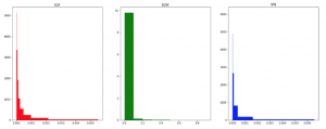
Figure 1: Data density with various binning methods on Liver Cirrhosis bacterial species abundance dataset using the same 10 bins. X-axis shows a value range of abundance.

Data binning or Data Discretization is a data processing method which transforms continuous value into discrete value. To discretize continuous values into “bins”, we need to determine “breaks” where indicates which bin these values belong to. “Breaks” are real values which can be 0.1, 0.35, etc. that are considered as “boundaries” of bins. Let say, we have an array of values including 0.000012, 0.02, 0.56, 0.92. We would like to divide 10 bins which own an equal width for each bin on a considered value range from 0 to 1. The width of each bin or interval width, in this case, is  = 0.1. The value range of the first bin is from 0 to 0.1, the second bin is from 0.1 to 0.2, etc. In our study, we do not consider the values of 0 (zeros), so values which are greater than 0 and lower than 0.1 (such as values of 0.000012, 0.02) will belong to the first bin while the second bin contains values which are greater than or equal to 0.1 and lower than 0.2. For other values with the computation as above, 0.56 will belong to the 6th bin while the last bin (10th bin) contains 0.92. The breaks as the example mentioned consist of 0.1, 0.2, 0.3, 0.4, 0.5, 0.6, 0.7, 0.8, 0.9. We also add 0 to the breaks to compare whether the values are greater than 0 to distribute values to bins. Metagenomic data can exist outliers that cause many wrong many prediction results by learning machine algorithms. Binning approaches are expected to improve the performance by reducing the effects of minor observation errors and to get rid of noise in the data.

This section will present various binning approaches which can be binning with equal width or equal frequency of values or basing on species abundance distribution of several considered species abundance datasets or simply only considering whether the feature exists in the sample or not (value > 0), namely Binary Binning. Some methods combining between binning approach and transformation with scaler algorithms are also presented.

3.1        Equal Width binning

EQual Width binning (EQW) divides and delivers continuous values to bins which have equal width. Each bin has the equal width

which is computed by Maxnumberofbinvalue−Min value in the range of [Min, Max] of the data. For instance, we would like to deliver original values to 5 equal width bins (k = 5) using a range of [Min=0,Max=1], then width of each bin is 0.1 (w = 0.1). The interval boundaries include Min + w, Min + 2 × w,…, Min + (k − 1) × w. The idea is simple but this method show improvements in prediction tasks.

3.2        EQual Frequency binning (EQF)

Equal frequency binning method cuts the data into n parts (bins) which each part contains approximately the same number of values.

The breaks are identified using the training set so the performance in the testing phase will be poor if the training set cannot reflect exact general data distribution of the considered disease. Breaks depend totally on data distribution so the width of each bin can vary significantly.

3.3        Binning based on species abundance distribution

SPecies Bins (SPB) is extended from EQW combining species abundance distribution conducted from 6 species abundance datasets in [1]. Authors in [1] presented breaks including 0,10⁻⁷,4 ∗ 10⁻⁷,1.6 ∗ 10⁻⁶,6.4 ∗ 10⁻⁰⁶,2.56 ∗

10⁻⁰⁵,0.0001024,0.0004096,0.0016384,0.0065536 for Species Bins. The first break ranges from 0 to 10⁻⁷ which is the smallest value of species abundance known in six species abundance datasets of CIR, COL, IBD, OBE, T2D, and WT2 [1]. The width of each bin is equivalent to a 4-fold increase from the previous bin.

3.4        Equal Width binning combining scaler algorithms

Some transformation algorithms applying to original data can be useful for binning. Standardization method is a widely-used technique for numerous machine learning algorithms to resolve the problem of different data distributions. Quantile Transformation (QTF), MinMaxScaler (MMS), and logarithmic computations scalers are considered to convert data before binning.

Quantile Transformation is implemented to combine with EQW in these experiments. QTF is considered as a robust pre-processing technique because it can reduce the effect of the outliers. Samples in test and validation sets which are smaller or larger than the fitted range then will be assigned to the bounds of the output distribution. Another algorithm illustrated in this study is MinMaxScaler, to make a comparison with QTF and logarithmic computations. MinMaxScaler converts each feature to a given range by (1) and (2) formulas:

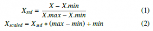
Functions which perform the transformation as above are now available in scikit-learn library.

As described in [1], metagenomic data usually follow the zeroinflated distribution. Data scaled with the methods of transformation based logarithm calculation reveal more normally-distributed. In this study, we use logarithm computation base 4 and base 100 for comparison.

3.5        Binary Bin

Binary Bin (B2) which can be considered as the one-hot encoding method, also is brought to compare. B2 indicates whether a feature is present or absent in a sample. If values are greater than 0, Bin 1 contains them. Otherwise, they are delivered to Bin 0 (with all values=0).

3.6        Data distribution Visualization of binning methods and scalers

Figure 1 shows various binning approaches on CIR dataset.

The breaks of EQF include 0,4 ∗ 10⁻⁰⁷,2.47 ∗ 10⁻⁰⁵,6.2 ∗ 10⁻⁰⁵,1.27∗10⁻⁰⁴,2.466∗10⁻⁰⁴,4.788∗10⁻⁰⁴,9.783∗10⁻⁰⁴,2.1484∗ 10⁻⁰³,5.5149 ∗ 10⁻⁰³. These breaks are approximate to SPB. We note that some first bins (with EQF) own high density with the width of these are rather small (4 ∗ 10⁻⁰⁷ for the first bin) while the width of the 9th bin is about 3.4 ∗ 10⁻⁰³. Similar results are exhibited for SPB. Width of each bin with EQW is equal, so we can see that the first bin contains most of the data.

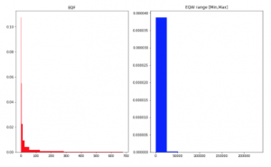
Figure 2: Data density on Crohn Read Counts dataset. X-axis shows a value range of counts with breaks using EQF and EQW on Min-Max range of training set.

For data type of counts, the values in features can be greater than 1, so SPB and EQW considering in a value range from 0 to 1 are not efficient for this type. EQW with a range between Min and Max values in the training set and EQF can work in this situation (Figure 2). Observed and conducted from Figure 2 for EQW method, we see that data distribution of metagenomic is the zeroinflated distribution, no matter what data is abundance or counts. However, a transformation with logarithm enables data to be more normally-distributed (Figure 3).

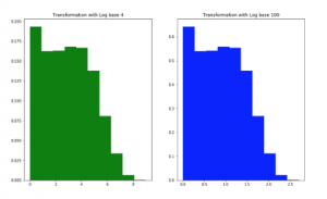
Figure 3: Data density on Crohn Read Counts dataset after transformation with logarithm base 4 and 100. The X-axis shows a transformed value range

The performance of the proposed binning methods will be evaluated in the next section (Section 4).

4. Experimental Results on Metagenomic data binning Approaches

To exhibit the efficiency of binning approaches on various machine learning algorithms, we present the results with a classic machine learning algorithm (Random Forest), Linear Regression and a famous deep learning technique that is Convolutional Neural Network on 1D data (CNN1D).

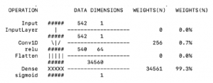
Figure 4: CNN1D architecture.

The algorithms of CNN1D, Linear Regression are both implemented using Adam optimization function, a learning rate of 0.001, and using an overall epoch of 500 along with a batch size of 16 and binary cross-entropy loss function. To reduce overfitting issue, we use ”Early Stopping” with the number of epoch patience of 5. The learning will stop if the Loss is not improved after 5 consecutive epochs. As conducted from [1], we should use a shallow deep learning architecture instead of deeper architectures, so the proposed CNN1D architecture includes a convolutional layer consisting of 64 filters of the size of 3, following by a max-pooling of size 2, and an activation function of ReLU [28]. The details of CNN1D are visualized in Figure 4.

Random Forests algorithm is a robust learning algorithm and widely-used in numerous studies related to bioinformatics tasks. In this study, Random Forest algorithm is deployed with 500 trees, nodes are expanded until all leaves are pure or until all leaves contain less than min samples split = 2 where min samples split is the minimum number of samples required to split an internal node.

The performance of each classifier is measured by an average of Area Under the Curve (AUC) and an average Accuracy (ACC) on 10-stratified-fold-cross validation repeated 5 times. The same folds are used for all classifiers, i.e. training and test sets were identical for each classifier. Besides, results are visualized by Boxplot to exhibit graphically depicting groups of numerical data through their quartiles. Our results are compared to state-of-the-arts including MetAML [18] on 6 species abundance datasets and Selbal [27] on 2 read counts datasets. MetAML [18] is a framework for metagenomic data analysis running on species abundance with classic machine learning algorithms such as SVM and Random Forest. MetAML performed the best with Random Forest; hence in comparison with our methods, we also run the classification tasks using Random Forest with the same parameters with MetAML. Selbal uses balance score to find good features, then fetching the features into Linear Regression algorithms for the prediction tasks.

We need to specify the value range to divide bins for binning approaches. In this study, the considered value range can be either [0,1] or [Min,Max] to divide bins for data. [Min,Max] means we consider the range covered by the minimum value and the maximum value of all features in the training set to bin the data.

We present the experimental results as followings. First, we show the disease prediction performance of all considered binning approaches (Section 4.1). Next, we evaluate and compare the differences in performance when we change the number of bins. Then, promising methods are compared with the state-of-the-art including MetAML [18] and Selbal [27].

4.1        Evaluation on different data pre-processing methods for metagenomic data

We compare the performance of various pre-processing methods based on binning approaches with three different widely-used machine learning algorithms including Random Forests (Figure 5), Convolutional Neural Network (Figure 6) and Linear Regression (Figure 7).

Figure 5 shows the prediction performance of the considered binning methods performed by Random Forests on 8 considered datasets. We compare the efficiency of different binning approaches (B2, EQF, EQW, SPB) and various scalers (Logarithms, Min-Max Scaler, Quantile Transformation). Except for Crohn dataset, there are not too significant differences in the performances of Random Forests algorithm with different approaches. In the chart, NA (“Not Available”) means the model running on the original data without using binning, so the value range for binning is also NA (for example, NA log4 NA, NA none NA, etc.). For CIR and OBE datasets, EQF without using scaler achieves the best performance. The average AUC for predicting CIR, OBE datasets using EQF none are 0.95582, 0.68238, respectively. For samples from COL dataset, the highest result is with QTF scaler. The datasets of Crohn’s disease, HIV, IDB achieve the best results with EQW binning combined with QTF scaler on the value range of [Min,Max]. The best AUC for Crohn’s disease dataset is 0.86976 and IBD obtains the best value at 0.88888 while HIV dataset obtains the best at 0.72438. The remaining 2 datasets including T2D and T2W using the binning method of EQW on the range of [Min,Max] without using scaler, reach the AUC best at 0.76286 and 0.80868, respectively. Crohn dataset shows worse results on the value range of [0,1]. It seems more appropriate because this dataset uses read count where the values are either equal 0 or greater than 1.

Figure 6 exhibits the results of CNN model on the considered datasets. As seen from the figure, binning approaches can outperform other methods. CIR dataset has the highest AUC value of 0.95986 while IBD dataset owns the best AUC value of 0.90894. Both two those results are evaluated with EQF without using any scalers. COL dataset obtains the best results with using the EQW combined Min-Max scaler on the value range of [Min,Max] of the training sets with AUC of 0.83732. Crohn’s gets the best result using QTF scaler with AUC of 0.85698. The prediction results on HIV disease using EQF without scaler on the value range of [Min,Max] peak at the best AUC value of 0.72788. OBE dataset has the highest AUC when we use the SPB approach. Two datasets of T2D, T2W running with EQW binning on the range of [0, 1] exhibit the best AUCs of 0.75746, 0.80238, respectively.

We also present performances of Linear Regression algorithm in Figure 7. As exhibited, the results are rather similar to mentioned previous two algorithms. CIR dataset obtains the best AUC value of 0.95870 with using EQF binning on the range of [0,1] while we achieve the best AUC of 0.83990 on COL with EQW. Original data of Crohn dataset being run by QTF scaler reaches the highest AUC value of 0.86884. Some results on other datasets are similar to CNN’s results.

From the shown experimental results, we notice that CNN, in general, achieves better results than using Random Forest and Linear Regression. Binning approaches appear to be more efficient to enhance significantly the performance with CNN and Linear Regression.

The methods of EQW on the value range [min, max] of training sets, EQF binning and scalers algorithms appear to be appropriate methods for the prediction tasks of HIV and Crohn’s disease where the values of features can be greater than 1. Comparing to the performance of the original data (NA none NA), these methods can give significant improvements.

4.2        Number of bins for Metagenomic binning

A comparison among the numbers of bins for binning EQW approach is presented in Figure 8. Average AUCs on each number of bins applying to 8 considered datasets are calculated to compare. The numbers bins of 5, 10 give average AUCs (on 8 datasets) of 0.8022450, 0.8011900, respectively while using 100 and 255 bins reveal AUCs of 0.7621925, 0.7471600, respectively. The binary bin approach reaches the average AUC of 0.7958750. As observed, the numbers bins of 5 and 10 obtain significantly better results compared to 100 and 255 bins. As shown from the average performance on the all considered datasets, data discretization with 5 bins

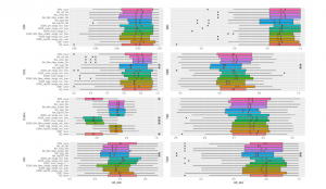
Figure 5: Different Methods Comparison using Random Forest. ”*” reflects significant differences compared to the best result on each dataset. ”X” reveals average performance on 10-fold cross-validation repeated 5 times. Methods names denote The binning method combining Scaler and data range for binning. For example,

NAnoneNA means no binning method or scaler is applied. Black Dots exhibit outliers in results.

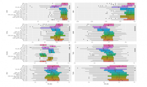
Figure 6: Different Methods Comparison using CNN. All symbols and stickers in the chart are the same as Figure 5.

We see that CIR dataset obtains the best AUC value is 0.9522 with 100 bins. Three datasets of COL, OBE and T2W reveal the best while IBD dataset achieves the AUC value of 0.88162 with 2 bins. ^{AUC values with 5 bins with AUCs of 0.83670, 0.69594, 0.80238,}

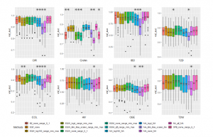
Figure 7: Different Methods Comparison using Linear Regression. All annotations in the chart are the same as Figure 5.

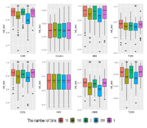
Figure 8: Performance of the various number of EQW bins using the CNN model. “*” reflects significant differences compared to the best result on each dataset. “X” reveals average performance on 10-fold cross-validation repeated 5 times.

respectively. Otherwise, prediction tasks on the diseases of HIV and art including MetAML [18] and selbal [27].

T2D with 10 bins give the best results.

In Table 2, we display the results using binning approaches of

4.3    State-of-the-art comparison                                   

EQW, EQF, SPB with a total of 5 bins and comparing state-of-the-art in average ACC and average AUC on 10-fold cross-validation To reflect the efficiency of binning approaches on metagenomic data,             repeated 5 times. Three datasets including CIR, OBE and T2W all we compare the proposed binning approaches to some state-of-the-    had better results than state-of-the-art. COL disease has only better

Table 2: Results Comparison of robust binning methods (the number of bins is 5 for EQW, EQF and SPB) and state-of-the-art (Selbal on HIV, Crohn’s disease and MetAML on other datasets) in average ACC and average AUC on 10-fold cross-validation repeated 5 times. The results formatted in bold text are better compared to the

state-of-the-art.

Datasets			CIR	COL	Crohn	HIV	IBD	OBE	T2D	T2W	AVG
	State-of-the-art	val acc	0.877	0.805	NA	NA	0.809	0.644	0.664	0.703	0.750
EQF	CNN	val acc	0.906	0.792	0.783	0.833	0.829	0.680	0.655	0.722	0.775
EQF	RF	val acc	0.887	0.808	0.813	0.816	0.810	0.657	0.675	0.720	0.773
EQW	CNN	val acc	0.883	0.785	0.739	0.827	0.851	0.668	0.667	0.707	0.766
EQW	RF	val acc	0.886	0.791	0.745	0.809	0.807	0.645	0.680	0.708	0.759
SPB	CNN	val acc	0.903	0.790	0.737	0.828	0.830	0.672	0.650	0.727	0.767
SPB	RF	val acc	0.883	0.785	0.739	0.827	0.851	0.668	0.667	0.707	0.766
	State-of-the-art	val auc	0.945	0.873	0.820	0.674	0.890	0.655	0.744	0.762	0.795
EQF	CNN	val auc	0.960	0.833	0.830	0.725	0.909	0.689	0.750	0.792	0.811
EQF	RF	val auc	0.956	0.866	0.868	0.703	0.872	0.682	0.754	0.781	0.810
EQW	CNN	val auc	0.952	0.837	0.775	0.718	0.881	0.696	0.757	0.802	0.802
EQW	RF	val auc	0.946	0.863	0.790	0.703	0.875	0.680	0.757	0.797	0.801
SPB	CNN	val auc	0.955	0.832	0.775	0.718	0.896	0.699	0.742	0.801	0.802
SPB	RF	val auc	0.952	0.837	0.775	0.718	0.881	0.696	0.757	0.802	0.802

ACC value when binning with EQF combined with Random Forest model (ACC value is 0.868). In Crohn’s disease, when performing the binning method with EQF combined with 2 models CNN (ACC value is 0.830) and Random Forest (ACC value is 0.868) both give better results than state-of-the-art. AUC values for HIV disease are better than state-of-the-art in all models and methods, but there is no ACC result in this disease higher than state-of-the-art. IBD has 5 good results when done with ACC values but only 2 good results for AUC. T2D has most of the results better than state-of-the-art, only when doing SPB method with CNN model (both ACC and AUC values) and when binning with SPB, CNN model with ACC measurements are lower than state-of-the-art.

5. Conclusion

In this study, we presented Met2Bin with various binning approaches using Equal with binning, Equal frequency binning, Species bins and binary bins to reduce the effects of minor observation errors and to get rid of noise in the metagenomic data. Scaler with QTF and logarithm transformation also show potential improvements in the data type of reading counts. In most cases, binning approaches and scaler algorithms can improve performance for machine learning algorithms.

The binning and scaler approaches are examined on a vast of datasets including different diseases and various data types (species abundance and read counts at genus or family or order levels). We can see that the proposed method can work on any value ranges. This research only takes into account unsupervised binning methods. Considerations on the labels of samples should be carried out in further studies.

As revealed from the performance of disease prediction, we can predict Liver cirrhosis, IBD with high accuracy while Obesity, HIV and T2D diagnosis are still challenges. Further research should investigate to improve those diseases.

In general, CNN produces better results than classic machine learning. However, the considered CNN architecture in this work is rather small and modest but its performance exhibits promising results. Further investigations on the CNN architectures should be considered to improve the performance. We also do not consider the labels of samples when we build the breaks for data binning. In the future, the research should consider and investigate the supervised binning approaches to evaluate whether those can be efficient or not on metagenomic data.

The binning methods are potential methods so that we can use such bins for converting numeric data and showing them in 2D images. A bin which represents the magnitude of value can be shown in the image with a specific colour. Binning techniques enable us to visualize bio-markers in images as well as to leverage advancements in deep learning algorithms for images to do prediction tasks.

The results and other materials of this work can be downloaded from https://github.com/thnguyencit/met2bin.

Conflict of Interest

The authors declare no conflict of interest.

1. Thanh Hai Nguyen, Jean-Daniel Zucker. Enhancing Metagenome-based Disease Prediction by Unsupervised Binning Approaches. The 2019 11th International Conference on Knowledge and Systems En- gineering (KSE-IEEE), ISBN: 978-1-7281-3003-3, pp 381-385. 2019.
   https://doi.org/10.1109 9295
2. Colorectal Cancer: Statistics Approved by the Cancer.Net Editorial Board. 2020. https://www.cancer.net/cancer-types/colorectal-cancer/statistics
3. Young-Hee Yoon, Chiung M. Chen; Liver cirrhosis Mortality in the United States: National, State and Regional Trends, 2000-2015. 2018. https://pubs.niaaa.nih.gov/publications/surveillance111/Cirr15 .htm.
4. C. Mathee et al. ;SURVEY AND SUM- MARY: Current methods of gene prediction, their strengths and weaknesses; p. 4103-4117.ISSN 0305-1048. 2002. https://doi.org/10.1093/nar/gkf543
5. Z. Wang, Y. Chen and Y. Li;A Brief Review of Computational Gene Prediction Methods; p. 216-221. ISSN 1672-0229. 2004. https://doi.org/10.1016/S1672- 229(04)02028-5
6. N.P. Nguyen et al.; A perspective on 16S rRNA operational taxo- nomic unit clustering using sequence similarity; ISSN 2055-5008. Nature. https://doi.org/10.1038/npjbiofilms.2016.4
7. M. Arumugam et al.; Enterotypes of the human gut microbiome; 473, p. 174-180. ISSN 1476-4687. 2011 https://www.nature. com/articles/nature09944
8. S. Park et al.; hc-OTU: A Fast and Accurate Method for Clustering Opera- tional Taxonomic Units Based on Homopolymer Compaction; 15, p. 441-451.
   ISSN 1545-5963. 2016. https://doi.org/10.1109/TCBB.2016.2535326
9. Wei ZG et al.: A Dynamic Multi-Seeds Method for Clustering 16S rRNA Se- quences Into OTUs. PubMed. 2019. https://doi.org/10.3389/fmicb.2019.00428
10. D. H. Huson, D. C. Richter, S. Mitra, A. F. Auch and S. C. Schuster; Meth- ods for comparative metagenomics; 10, p. S12. ISSN 1471-2105. 2009. https://doi.org/10.1186/1471-2105-10-S1-S12
11. L.-x. Chen, M. Hu, L.-n. Huang, Z.-s. Hua, J.-l. Kuang, S.-j. Li and W.-s. Shu; Comparative metagenomic and metatranscriptomic analyses of microbial communities in acid mine drainage; 9, p. 1579-1592. ISSN 1751-7370. 2015. https://doi.org/10.1038/ismej.2014.245
12. S. Nayfach et al.; Toward Accurate and Quantitative Comparative Metage- nomics; 166, p. 1103-1116. ISSN 0092-8674. https://doi.org/10.1186/1471- 2105-10-S1-S12
13. S. M. Dabdoub et al.; Comparative metagenomics reveals taxonomically idiosyncratic yet functionally congruent communities in periodontitis; 6, p. 38993. ISSN 2045-2322. https://doi.org/10.1038/srep38993
14. K. Sedlar et al.; Bioinformatics strategies for taxon- omy independent binning and visualization of sequences in shotgun metagenomics; 15, p. 48-55. ISSN 2001-0370. 2016. https://doi.org/10.1016/j.csbj.2016.11.005
15. H. Soueidan et al.; Machine learning for metagenomics: methods and tools; Metagenomics 1. 2017. https://doi.org/10.1515/metgen-2016-0001
16. G. Ditzler et al.; Forensic identification with environmental samples; IEEE In- ternational Conference on Acoustics, Speech and Signal Processing (ICASSP). 2012. https://doi.org/10.1109/ICASSP.2012.6288265
17. G. Ditzler et al.; MultiLayer and Recursive Neural Networks for Metage- nomic Classification; IEEE Transaction Nanobioscience 14, p. 608-616. 2015. https://doi.org/10.1109/TNB.2015.2461219
18. E. Pasolli et al.; Machine Learning Meta-analysis of Large Metage- nomic Datasets: Tools and Biological Insights; PLoS Comput. 2016. https://doi.org/10.1371/journal.pcbi.1004977
19. D. Fioravanti, Y. Giarratano, V. Maggio, C. Agostinelli, M. Chierici, G. Jurman and C. Furlanello; Phylogenetic convolutional neural networks in metagenomics; 19, p. 49. 2018. ISSN 1471-2105. https://doi.org/10.1186/ s12859-018-2033-5
20. D. Reiman, A. A. Metwally and Y. Dai; PopPhy-CNN: Ation Neural Net- works for Metage- nomic D Phylogenetic Tree Embedded Architecture for Convoluata. 2018. http://biorxiv.org/lookup/doi/10.1101/257931
21. F. Celesti, A. Celesti, J. Wan and M. Villari; Why Deep Learning Is Changing the Way to Approach NGS Data Processing: a Review; ISSN 1937- 3333. 2018. https://doi.org/10.1109/RBME.2018.2825987
22. J. Ren et al.; Identifying viruses from metagenomic data by deep learning. 2018. http://arxiv.org/abs/1806.07810
23. Subrata Saha, J. Johnson, S. Pal, G. M. Weinstock, S. Rajasekaran, MSC: a metagenomic sequence classification algorithm, Bioinformatics; vol.35, 17,p. 2932-2940. 2019. https://doi.org/10.1093/bioinformatics/bty1071
24. Jolanta Kawulok, M. Kawulok and S. Deorowicz; Environmental metagenome classification for constructing a microbiome fingerprint. Biol Direct 14. 2019. https://doi.org/10.1186/s13062-019-0251-z
25. Lo Chieh, Marculescu, Radu; MetaNN: accurate classification of host pheno- types from metagenomic data using neural networks. CM University. Journal contribution. 2019. https://doi.org/10.1186/s12859-019-2833-2
26. K. Sedlar et al.; Bioinformatics strategies for taxonomy independent binning and visualization of sequences in shotgun metagenomics; 15, p. 48-55. ISSN 2001-0370. 2018. https://doi.org/10.1016/j.csbj.2016.11.005
27. Rivera-Pinto J, Egozcue JJ, Pawlowsky-Glahn V, Paredes R, Noguera- Julian M, Calle ML. Balances: a New Perspective for Micro- biome Analysis. mSystems. 2018;3(4):e00053-18. Published 2018 Jul 17. https://doi.org/10.1128/mSystems.00053-18
28. Abien Fred Agarap. Deep Learning using Rectified Linear Units (ReLU). 2018. https://arxiv.org/abs/1803.08375

(Click Here)

(Click Here)