1. Introduction

One of the most serious problems found in many chemical industry and its components degrade over time (e.g. wear, corrosion, erosion and fatigue). Among the components, we consider the pipelines, which are widely used in industrial plants networks and water distribution networks. The pipeline system are considered, one of the components more susceptible to failure in many industrial applications and that deteriorate over time. This deterioration occurs as a result of the damaging effects of fluid mixture produced from a reservoir or caused by the environment effects. Which is called crud fluid and it contains a variety of substances of different chemical structure that include hydrocarbon and non hydrocarbon components. Furthermore, the surrounding environment may cause a corrosion effect of pipe cross-section. As mentioned above the wax layer will build up in layers and can block the pipeline. Which can be reduce the pipeline reliability and safety level. This paper is an extension of work originally presented in conference name [1]. The aim of this paper is to present an approach to quantifying the reduction in reliability and safety. However, we designed a new technique for predict the remaining useful life time for clogging pipelines at point in time and a specific distance. We will focus our study mainly on cross section clogging pipelines. It may become a serious problem as a pipeline ages. Based on literature, several theories have been proposed to explain the reliability and the safety of pipelines circumferential strength. It follows that a failure level threshold is dened for stochastic deterioration process model, which must not be exceeded for economical or security reasons. Obviously, the accumulated deposit on the pipeline wall causes the growth of a thickness of wax layer, leading to higher pressure drop and/or decreased flow rate [2]. Through periodic inspection, the growth of wax layer defect can be monitored, it follows that the reliability of pipeline system can be improvement. The loss of efficiency of the pipeline is then viewed as a change in the open loop system. Improvement reliability and safety of pipeline can be studied based on prognostic analysis. It can be defined as the prediction of future characteristic of the system such the Remaining Useful Life. Current research on diagnosis and prognostic are based on estimation the non observable system state. One of the most technic used is the stochastic filtering approaches, which gives an estimation of the system state recursively. Therefore, we can benefit from these, which give an estimation on-line with reliable performances for the parameters of a given model or a degradation path. However, Kalman Filtering (KF) and Extended Kalman Filtering (EKF) have been successfully applied to fault prognosis respectively in linear system dynamics model and nonlinear system dynamics model [3, 4]. According to the literature,[5]-[8]about degradation modeling can be mathematically described with a continuous process in terms of time, Lu[9] use the convex degradation model for the growth rate of fatigue cracks. Wang [10] studies a class of Wiener processes with random effects for degradation data.

The remainder of this paper is organized as follows: In section 2, a two tank system modeling and it treats the stochastic deterioration in pipeline and explains why the Wiener process is the most appropriate candidate for clogging evolution. Section 3 is devoted to diagnosis and analysis the failure in pipeline system based on the EKF algorithm. Section 4 discusses two methods for estimation of the RUL, the first one is used to predict the RUL by EKF and the second method used Monte Carlo simulation to estimate the RUL. Finally, section 5 makes some concluding remarks.

2. Degradation Modeling in Pipeline System

Theoretically, in our case for modeling the movement of small particles in uids, which can causes an additive accumulation of wax overtime. Therefore, a characteristic feature of this process in the context of structural reliability is that a pipelines resistance alternately increases and decreases. For this reason, the Brownian motion is adequate for this deterioration modeling which is no monotone. We can assume that degradation increment increases in time with random noise. In the literature, several theories have been proposed to describe the phenomenon of degradation by a stochastic model or a deterministic model [11, 12]. Several publications have appeared in recent years documenting the degradation evolution that can be described by Wiener process or gamma process [13]. In the following work, we consider the stochastic failure model. To solve this problem, many researchers have proposed various methods of modeling, mainly the stochastic model can be continuous or discrete [14, 15]. Wiener processes are widely applied for modeling the degradation process in engineering systems. Many physical phenomena are described by the Wiener processes, when the cumulative damage is non-monotonic. For example in our case, clogging or partial blockage in cross area pipeline is then viewed as a non-monotonic degradation processes. According to the literature the Wiener process with a linear drift is frequently used to model the non monotonic degradation process [16, 17]. Much research on the non monotonic effect has been done about degradation process based on the nonlinear model, which was proposed in many literatures [10, 18, 19].

2.1        A Two Tank System Modeling

In our study, we consider a two tank system with pipeline. However, the section area of the rst tank is noted by A₁ and the second one is noted by A₂. The uid is assumed as incompressible (ρ is assumed constant), which is pumped into the rst tank at the top by motor pump . Through the pipeline, the outow from the rst tank fills the second tank. The overall tank system is shown in Figure 1. We assume the fluid level of tank1 and tank2 are measured by a level measurement sensor and controlled by adjusting the pump motor control input not shown in this case. The aim of this modeling is to control the state of the pipeline and to intervene before having the failure. In the following we assume an abrupt change at time and a given distance in this cross-sectional area of the pipeline, which is then viewed as a change in the tank fluid level. From this modeling it can be given a mathematical model in engineering system. In this way we can simulate the evolution of the clogging in pipeline, obviously we can improving the pipeline reliability based on the estimation of the RUL.

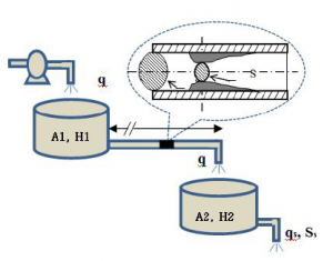
Figure 1: A double tank with pipeline

Table 1: Nomenclature

Parameter	Description
Ai	Tank cross-sectional area (i=1,2)
Hi	Fluid level (i=1,2)
p0	Atmospheric pressure (Pa)
p1	Pressure at the bottom (Pa)
%	Fluid density (Kg/m3)
g	Acceleration of gravity (m2/s)
Z0	Level fluid in the upper tank (m)
Z1	Level fluid at the bottom tank (m)
V	Fluid velocity (m/s)
h	State level at time t in tank (m)
S s,S i	Pipeline area (m2)
S c	Pipeline area clogging(m2)
q	flow rate (m3/s)

Let us describe the following failure mode encountered in petrochemical industrial applications these are:

1. clogging and partial blockage in pipeline cross section. Which arecaused by impurities and an additive accumulation of wax overtime, see Figure 3.
2. Decreasing pump performance due to cavitations,
3. Dry running.

To control pressure losses, clogging, leaks, corrosion in the pipeline. We assume that are two pressure sensors between the upstream and downstream tank. This is illustrated in Figure 2. We will make the following assumptions: The logging is supposed located at distance (d < L) and the pressure losses are neglected along the pipeline.

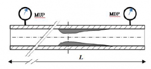
Figure 2: showing the deposit profile of wax

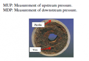
Figure 3: Clogging inside the pipeline

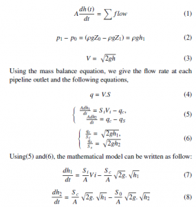
In order to describe the overall tank fluid level control system, we have some assumptions: The fluid is incompressible (ρ is constant), the temperature distribution of the incoming fluid is assumed constant, the flow rate is considered permanent. Under all these considerations, we use the mass balance equation, Torricelli rule and Bernoulli rule it follows that the process can be described by the following equations,

The implementing of equation (7) and equation (8), we can be rewritten the discredited model for a sampling period Te.

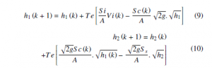
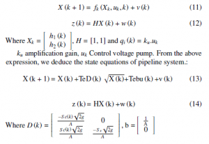
The state equation has the nonlinear terms (a square term), it follows that a nonlinear system. If we consider the process noise v(k) and the measurement noisew(k), the state equation X(k +1) and measurement equation z(k) can be written as follow:

2.2        Wiener process for degradation modeling

For modeling the stochastic deterioration process, we can use Brownian motion with drift, as far as the author knows, the Wiener process was applied frequently in many works [14, 17]. In this work, for more control the evolution of pipeline state, the monitoring pressure differential ∆p can be designed as a degradation indicator in pipeline [15]. In the following, the Wiener process is used to model the clogging damage in pipeline. Which is considered a no monotonic degradation processes. However, we assumed that the degradation increases linearly in time with random noise. In practice, the degradation processes of pipeline systems are affected by partial blockage or clogging formulated by the crud fluid and external operating environments or loads. Let’s call again the properties of Wiener process to model the pipeline clogging evolution, in order to lifetime and reliability analysis. 1. X (0) = 0;

2. The process {X(t)} has stationary and independent increment,
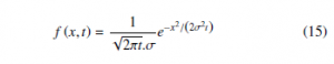
3. The process {X(t)} is assumed normally distributed with µ = 0 and variance σ²t for any t > 0. Considering the time variables t,u > 0, the random variable X (t + u) − X (u) and X (t) − X (u) for t > u, have a normal density with mean 0, and variance σ²t and σ² (t − u) respectively, In this way we define the probability density function as f (x,t) of Pr {X (t + u) − x(u) ≤ x} = Pr {X (t) ≤ x} is as follows

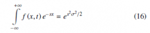
and its Laplace transform is

When σ = 1,B(t) ≡ X (t)/σ, is a standard Brownian motion because V {X (t)/σ} = t. For any 0 ≤ t₀ < t₁ < … < t_n < t, using the properties of independent and stationary increments, it is evident to write the probability

In this way, we assume that the process has a Markov property. Hence, its distribution function can be written as follows:

Where the increment X (t) − X (t_n) has a pdf with mean µ = 0 and variance σ² (t − t_n) for any t > t_n, that does not depend on t_n.

Where B(t) is a standard Brownian motion representing the stochastic dynamics of the degradation process, then Z (t) is called a Wiener process with drift parameter µ and variance σ². The pipelines failure is caused by the fluctuation of the fluid pressuredepression along the time P_min and P_max, that are repeated within an interval of time. Moreover, in [12]we deduce a minimum wax removing pressure. Obviously these pipelines are unfortunately usually designed for ultimate limits resistance. It is noted here the evolution of the internal pressure can be caused a stochastic stress in cylindrical pipeline. Moreover, in the work [5] and [19] are used a nonlinear Wiener process with random effects to model

the degradation process in pipeline. A nonlinear Wiener process aims to model the heaping and movement of small particles in fluids with tiny fluctuations in pipeline. To assess the severity of the clogging in pipeline system and its impact on the residual life, it is required to analysis the degradation process characteristic. Therefore, the pipelines degradation can increase or decrease gradually under time. From now on we assume that the small increase or decrease for degradation pipeline over a small time interval be have similarly to the random walk of small particles heaping in cross sectional pipeline. Furthermore, the random effects are widely used in [10], [18] and [19] extended the degradation model in (19) to the following form:

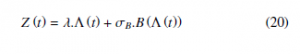
Where, λ: is the drift parameter

Λ(t): is a positive non decreasing function, we can use the timescale transformation function Λ(t) = t^θ and Λ(t) = e^θt − 1

σ_B: is the diffusion parameter,

B(t): is the standard Brownian motion.

If Λ(t) = t is a positive function, the nonlinear model becomes a linear model given by (19).

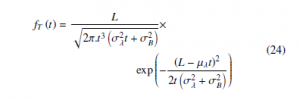
However, a fundamental problem related to this kind of degradation models of nonlinear Wiener-process. Actually, nonlinearity and stochastically are two important factors contributing to the degradation processes of complex systems. When the degradation process Z(t), t > 0 hits a failure threshold value L of the item was considered. The item’s lifetime T is defined as:

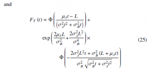
According to the concept of the First Hitting Time, it is evident, when the Wiener process path reaching a threshold level L, it can be obey an inverse Gaussian distribution. Obviously, when we consider the nonlinear degradation process as shown in (20) and the drift parameter λ is considered a random effect variable given by λ ∼ N (µ_λ,σ_λ). Moreover, according to [18] the probability distribution function (pdf) of the life time is given by (22) and similarly, the cumulative distribution function (CDF) of the life time is given by (23).

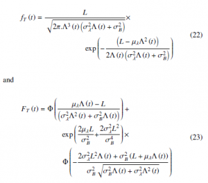
when we consider the linear degradation process as shown in (19) and the drift parameter λ is considered a random effect variable given by λ ∼ N (µ_λ,σ_λ). Then, the probability distribution function (pdf) and the cumulative distribution function (CDF) of the life time are given by:

2.3        Parameters Estimation using MLE

The Maximum Likelihood Estimation (MLE) is the most widely used. It is a method of estimating the parameters of a model. This maximizes the agreement of the selected model with the observed data. We assume that Z_i,j is a degradation indicator measurement (In this case the pressure differential see Figure 2) at the i^th items (We assume many pipelines are observed) at time j,where i = 1,2,3, N and j = 1,2,3,r, r is the last observation time. The degradation paths is based on linear Wiener process with parameters (µ,σ) and that are assumed the same for all items. For each increment

∆Z_i,j = Z_i,j+1 − Z_i,j of each item follows a normal distribution N µ∆t_i,j,σ²∆t_i,j. We assume that increment ∆Z_i,j is independent, identically components. Similarly it is assumed normally distributed for all. Now we can derive the density function of Brownian motion process, which is given by:

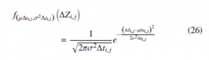
Z is a Markovian process, then the maximum likelihood estimator can be used. The parameters vector θ = (µ,σ) can be evaluated once we know the transition density function of Z. According to the measurements of degradation for each item i,

The degradation measurements vector are independent, then we can write, l(θ) = ln(∆Z₁,…∆Z_N)

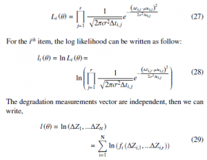
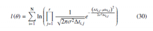
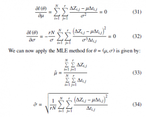
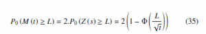
of increments, that is corresponding to each item, and f/l(θ) is the pdf divided by log likelihood of increments corresponding to all increments. In this way we obtain, we write the MLE θˆ = (µ,ˆ σˆ ) are found by maximizing l(θ), and using the partial derivative of the log likelihood function of (24), by respecting the derivation variables µ and σ, from this we deduce these equations,

2.4        First Hitting Time Concept and RUL Distribution

Based on the work presented in [20]-[22], the RUL of a system is dened as the length from the current time to the failure time. If we consider the random variable T as a stopping time for B(t), t ≥ 0, and for any t, it follows that to decide whether T has occurred or not by observing the path of B(s), 0 ≤ s ≤ t. For any t the sets {T ≤ t} ∈ F_t and given a level threshold L, the time of reaching this level could be more than once due to the random nature of Wiener process Z (t). In the following, we provide the computation of a first passage time hits level threshold T_L and the RUL distribution of Wiener process paths. Suppose T_L the first passage time of Wiener process Z (t) hits level L, if the maximum of Z (t) at time t is greater than L, then the path of Wiener process took value L at some time before t. Let consider T_L the rst time when the degradation path Z (t) reaches the threshold level, it follows that, we deduce the distribution of the maximum and the minimum of Wiener process on

[0,t]. Mand m(t) = min Z (s). identically , the 0≤s≤t distribution of the first hitting time of L, T_L = inf {t > 0 : Z (t) = L}. From Theorem [22], and for any L > 0 ,   !!

Proof: For the events M (t) ≥ L and T_L ≤ t are the same. When the maximum of Wiener process at time t hits a failure threshold L. If Wiener process took value L at some time before t, therefore the

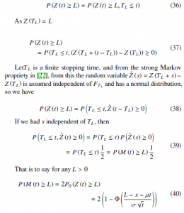
In reliability engineering , there are some researches involving the degradation based failure time T_L prediction for a component. Which is defined as the time at which the degradation path first reaches a threshold L. However, the distribution of the first passage time T_L plays an important role for predicting the remaining useful lifetime. Furthermore, RUL is often used as a decision indicator in the optimal maintenance strategies. According to [23], the inverse Gaussian distribution can be used to calculate the probability density function of the conditional rst passage time, when the degradation path is modeled by a Wiener process with positive drift. According to what is said before, let T_L can be the first passage time for a fixed threshold L > 0 by Z (t) which is the linear degradation process given in (19). Then T_L can be considered as a random variable described by the inverse Gaussian distribution as follow

T_L ∼ IG _µL,_σ^{L 2}. We should first mention inverse Gaussian distribution (IG) is a two parameter continuous distribution given by its density function as follow:

The mean µ > 0 and the shape parameter λ > 0. If we consider a random variable X which is governed by the inverse Gaussian distribution and can be written as follow X ∼ IG (µ,λ). However, the inverse Gaussian distribution describes the probability density function of the conditional rst passage time, when the degradation ∼ IG  _µ  ^{L 2} path reaches a level L. Then T_L ^L, _σ has inverse Gaussian distribution, so put these parameters into(35). Therefore, we have probability density function given by:

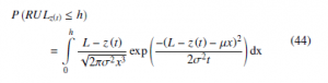
Given (36), it is possible to calculate the RUL distribution. If we take the observing data from the degradation process at time t, which is at position z(t), then the probability that RUL is less than a predened period h can be written as follow:

3. Diagnosis in pipeline using EKF

The suboptimal filter known as the Extended Kalman filter (EKF) is frequently used for non-linear state estimation problems. Since (13) and (14) that represent the model of pipeline system, that is nonlinear model. Before applied the EKF algorithm, we must linearize the state equations around the actual value of state estimated for each time step. A linear approximation process is done by using a Taylor series approximation. According to (11) and (12), we carried out the non-linear model of the pipeline system. From now on we apply the Taylor series approximation, in order to linearize the functions that given by equation (13) and equation (14)

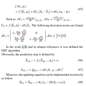
It is interesting to consider the error in the prediction of z_k from its past z_k−1. This error is known as the prediction residual on the innovation. This latter term comes from the fact that we can write:

The simulation data are taken from [25, 26] are given in Table 2.

Table 2: Nomenclature

Physical parameters	Description
A1 = A12 = A = 16(m2)	Identical sections for the two tanks
S 0 = 1/32(m2)	Tank outlet section N2
S i = 1/4(m2)	Tank outlet section N2
g = 9,81(m/s2)	Acceleration of gravity
T = 5(s)	Sampling period
S max = 1/4(m2)	Section of the pipe linking the two tanks
N = 100	Time (Year)
H1(1) = 0.5(m)	Level of the fluid in the first reservoir
H2(1) = 0.01(m)	Level of the fluid in the second reservoir
qi = 5(m3/s)	Flow rate

The numerical value of state noise for simulation are v =

Q.rand(1,n) and Q = diag(0.002,0.05,0.0001) The numerical value of measurement noise for simulation are w = R.rand(2,n) and R = diag(0.01,0.01).

4. System without Fault (No clogging)

According to the EKF algorithm given by (46) and (52), we illustrate and show the simulation results through a two tank system without degradation process. These simulation results are given by Figure 4 and Figure 5. According to the algorithm of EKF given by(46)-(52), which contains the fluid level and flow rate we can generate the statistical residual. According to the estimated value of level tank, it is possible to quantify the influence of wax deposition action. The simulation results as shown in Figure 4 and Figure 5. However, the pressure and flow rate in pipeline system are commonly measured in order to monitoring the characteristic pipeline system. These equations in algorithm of EKF incorporate a measurement value into a priori estimation to obtain an improved a posteriori estimation. The simulations results were carried out in the absence of clogging in pipeline system to show the fluid level evolution in two tank in Figure 4.

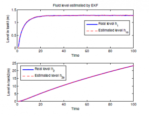
Figure 4: Fluid level in Two Tank system

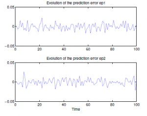
Figure 5: Residuals without faults(No clogging)

Consider Figure 5, which plots the residue observed from EKF for diagnosis, that indicates the system is no faulty. Moreover, it shows the filter performance measures in terms of the innovation sequence. We know that if the filter is working correctly, then the innovations have a zero mean Gaussian white noise with a covariance (S _r). However, we can verify that the filter is consistent by applying the following two procedures. Check that the innovation is consistent with its covariance by verifying that the magnitude of_√

the innovation is bounded by ±2      S _r . Verify that the innovation is unbiased and white.

The statistical characteristics of the residual without faults are given in Table 3:

Table 3: The statistical characteristics of the residual

Residual	Mean	Standard deviation
r1	µ1 = −0.000242	σ1= 0.0087
r2	µ2 = 0.0000321	σ2= 0.0102

Figure 6: Residuals statistical characteristics

4.1        System including clogging by Steps

In order to valid the EKF algorithm for dynamic failure estimation. Consider Figure 2, which shows the deposit profile of wax. We will be interested in clogging pipeline, that is assumed at distance d projected on the longitudinal axis (d < L), where the clogging can form a critical region of stress concentration and L is the length of the pipeline. In practice, this type of defect is unobservable and no measurable. For this reason, we consider two pressure sensors to control the increase or decrease the pressure downstream and upstream of the obstruction. Before use the degradation model by Wiener process that can be assumed and described by (n) steps to model the cumulative damage in pipeline. The model of degradation by steps can be described by (53), this results in a decreasing of cross sectional area and it model a clogging evolution in pipeline.

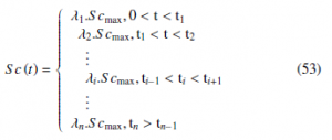
where 0 < λ_i ≤ 1, is a ratio between Sc(t)/Sc_max, see Figure 2. Thus, t_i−1 and t_i denote the initiative and terminal time under cumulative wax step respectively. However, in the following we have n = 3 steps, then λ₁ = 0.3, λ₂ = 0.5 and λ₃ = 0.7. Which, the first clogging level is assumed to occur at time t = 30 unit of time.

For a given form of evolution clogging level in cross-sectional area in pipeline Figure 9 and according to the EKF algorithm, it follows that the fluid level in tank1 and tank2 are affected by this clogging. Furthermore, the quality of the state estimation of the deposit profile of wax is accepted and well. The EKF algorithm is used to estimate recursively the pipeline system state, when we consider a deteriorating system with noisy measurement of h₁ and h₂. Figure 7 shows the fluid level evolution in two tank system. Moreover, Figure 8 depicts the prediction errors, which contains a statistical information for diagnosis.

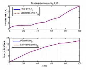
Figure 7: Fluid level in two tank

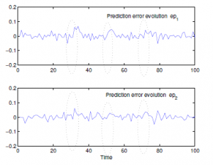
Figure 8: Residuals with three steps of faults

Consider Figure 9, which plots section degradation prole estimated by EKF. If we compare these results with Figure 4 and Figure 5, we can show the effect of clogging pipeline in the characteristics of pipeline system. One can notice that the performance of our proposed methodology of estimation and failure diagnosis are perfectly adopted. For a better lecture of Figure 9, we can conclude that the EKF algorithm is applied very well in order to estimate the state of the cross-sectional area in pipeline.

The problem consists to model the evolution of the wax in pipeline and to determine the minimum cross-section area which corresponds to a maximum pressure. That can cause a crack or an explosion of the pipeline system. For more reality and improve the clogging damage model, it is more appropriate to describe the type of failure with a continuous process.

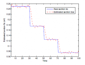
Figure 9: Section profile estimated by EKF

From this Figure 10, it can be seen that random evolutions of the internal section Sc(t) of the pipeline for a given distance (d < L). The time at which the prognosis is made it can be noted by t_pro. However, the remaining residual life of the pipeline system at t_pro will be noted RUL_tpro . It equals to the time elapsed between RUL_tpro and the moment when the pipeline system is failed. Noted that T be the date of failure, then the RUL prediction at the time of prognosis is assumed as a random variable which can be defined for t_pro < T (see Figure 10).

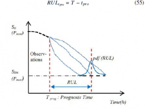
Figure 10: Remaining Useful Lifetime prediction

S _lim : Minimum value of Sc, when a lower value, there will be an explosion in pipeline, which can dene the threshold level. According to the literature [2, 27], who presented models for evaluation of the wax appearance at given point. From the authors work [28, 29], we can define the specific criterion for pipeline resistance as follow.

where

Sy : is the yield strength of the pipe material (MPa).

P_max: flow strength of the pipe material (MPa)

5. RUL Predicted by EKF and Monte Carlo simulation

The main objective in this section is to present an approach to evaluate the reliability. However, the RUL for deteriorating pressurized pipelines at any distance d and time t require to modeling this degradation process and predicted its evolution on line. We will focus mainly on cross-sectional area of pipeline, where the deposit profile of wax is shown in Figure 2. Based on paragraph (2.2) the degradation process models can be applied easily. From (19),the evolution of cross-sectional area of pipeline can be described by new form of Wiener process.

In order to assess clogging pipeline evolution, there are many techniques for estimation, KF and EKF is the most widely used for linear and non linear systems. Theoretically, we can estimate the RUL of a pipeline containing wax defects using two techniques EKF and Monte Carlo simulation.

5.1        RUL Predicted by EKF

In order to predicted the RUL by EKF that is computed using two steps the first one requires to estimate the clogging level evolution on cross-sectional area Sc(t) of pipeline, trough using the EKF algorithm for non linear system. The second require to use the estimated path of the clogging level and using (44) it may be evaluated the RUL cumulative distribution function. However, the prognostic of degradation path estimated by EKF and illustrated in Figure 12 is used. For a predefined period h and given the current degradation status (Time,Sc(t)), we can calculate the RUL distribution. For example from Figure 12, we are taken three points of current degradation path M₁(20,0.230), M₂(30,0.222) and M₃(40,0.215). Figure 13 depicts the cumulative RUL distribution in each point Mi. However, the red curve M₁ is the RUL distribution when monitoring time is 20 unit of time and 0.225 current level degradation. As we can see, the later the observing time, the higher possibility that the cumulative wax in cross-sectional area Sc of pipeline would within the predened monitoring time period.

For evaluation of RUL distribution, a philosophy of RUL estimation based on first passage time distribution, which is given by (44) in paragraph(2.4). In order to analysis the impact of Wiener parameters in degradation path, we demonstrate that with Matlab simulation. However, when µ is small in comparison with σ , we conclude that the drift has a greater impact on the Winer process. Conversely, if σ is small in comparison with µ , then noise dominates in the behavior of the Winer process. For more analysis, we generate ten realizations of Sc paths with µ and σ are estimated before. From (27) and (28), we can estimate the parameters corresponding to the data set. Using the MLE method the estimated parameters are given by:µˆ = 0.1525 and σˆ = 0.052. In the first time, we apply the EKF algorithm in Section 3. In order to predict the systems future state using (40-44), that enable to use the system information, through the measurement value, measurement error and system noise, it is possible to obtain a trend optimal estimation of the pipeline system state. Therefore, EKF is a recursive algorithm used for estimation, which needs to save the system state value and covariance matrix at the last time every step of estimation. For level value of degradation process path at unit of time, it is possible to predict the RUL of the pipeline system. The failure threshold value is set to respect the criterion of reliability and safety given in literature [28, 29].

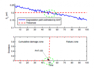
Figure 11: Degradation paths of Sc

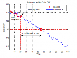
Figure 12: RUL prediction by EKF

Use the criterion in (56) to prove the pipeline system reliability. For example, for Sc_lim = 0.2(m²) obviously, the simulation results are shown in Figure(11) and Figure(12). That can give more information about prognostic. Consider Figure (11) which plots the degradation path of Sc, which is predicted by EKF algorithm. Given a threshold level Sc_lim, we can make decision between two hypothesis at time t = 50 unit of time, working zone and failure zone. Figure (12) illustrates the RUL prediction by EKF algorithm. When the path of Sc exceed the failure threshold at t = 55 unit of time, then we can compute the RUL from time of prognostict_pro = 20 unit of time until failure time. However, from (55) the RUL = 55(unit of time).

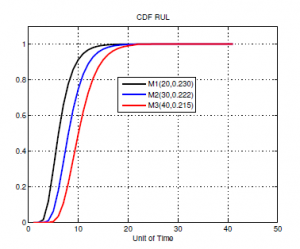
Figure 13: CDF of RUL

5.2        RUL Estimated by MC

The second method requires to generate many paths by Monte Carlo simulation and according to paragraph (2.4) we can evaluate the first hitting time and plot the RUL pdf. Using the Wiener model to generate some paths describing the true degradation process with parameters estimated before µˆ = 0.1525 and σˆ = 0.052. After that, we apply Monte Carlo simulation for a given threshold level to depict the RUL distribution. For more analysis, we generate the degradation paths of Sc using the presented approach based on Wiener model, we carried out several numerical simulations including the procedures of initial parameters estimation. Moreover, assume that Sc is simulated randomly for N = 10 realizations independent and identically tested and that are based on Wiener process with positif drift. In order to analysis the degradation process evolution, we simulate the testing data set using Matlab see Figure 14 and Figure 15. For simplicity and reasons of understanding the evolution of the degradation process, we simulate the first path with mean and variance parameters above and initial condition of Sc = 0.25m².

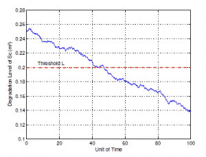
Figure 14: Degradation path of Sc

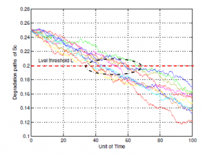
Figure 15: Degradation paths of Sc by MC (N=10)

In the following, we are taken N = 50 and N = 100 random samples are generated and we want to gure out the time when the degradation paths hits the failure threshold L = 0.2(m²). It follows that the distributions of first hitting time computed by Monte Carlo simulations, which are compared with analytical function of FHT in (42) as can be seen from Figure 16 and Figure 17. We can say that the analytical function of FHT based on Wiener process approximately pick up the true value in degradation process. However, it is not very reasonable to make such deterministic conclusion only according to gures results. An advanced evaluation need to be carry out to judge the accuracy of the proposed method and the model of degradation process. Nevertheless, there are some relevant problems to be addressed.

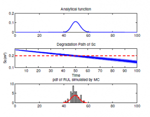
Figure 16: First Hitting Time and pdf RUL (N=50)

However, the choice of the initial parameters µ and σ of the degradation process is important for evolution of the Wiener dynamic drift. For this reason, a simulation with Matlab demonstrate that when µ is small in comparison with σ, then we conclude that drift has a greater impact on the dynamic of Wiener process. Furthermore, if σ is small in comparison with µ, then the noise dominates in the behavior of the Winer process. But it is very obvious from these gures that the Wiener processes are more spread out when its parameters are fluctuated. Moreover, it appears that the paths has regions where motions looks like they have decreased trend with random uctuations. It seems to me in this practical case, the degradation does not follow a linear drift.

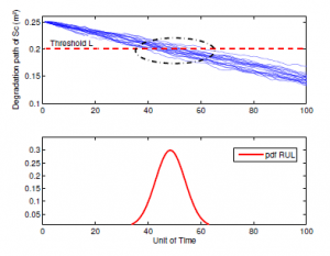
Figure 17: Monte-Carlo Simulation and pdf RUL (N=100)

Figure 18 shows the actual pdfs RUL at different observation. The first curve in the figure is the pdf RUL when monitoring time is t = 0 unit of time and the last curve shows the pdf RUL when monitoring time is t = 5 unit of time. It is clear that, the latter observing time, the rather that pipeline would have clogging higher possibility. Similarly, we can estimate the mean of the RUL as an useful input for a preventive maintenance activity.

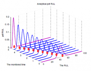
Figure 18: Analytical pdf of the RUL prediction

6. Conclusion

In this paper, we have proposed a new idea that allows to model the degradation process in two tank system. We have focused our modeling particular in pipeline clogging component. We only consider a Wiener process without random effects has a linear drift. But in practice, a nonlinear model may be more appropriate for complex system. Based on the Wiener process model, the unknown parameters in this model are estimated using the MLE approach. However, at the beginning of modeling we have used a simple model to describe the cumulative damage which causes by the small particles in crud fluid in pipeline system. In this context, we have assumed the clogging of cross sectional area of pipeline by walk steps. By using the Extended Kalman Filter algorithm, we have effectively estimated the state parameters system. There fore, the EKF algorithm has been successfully applied to predict recursively the Remaining Useful Life Time of the pipeline containing wax defect. Based on the concept of the First Hitting Time, the Monte Carlo simulation method is used to estimate the probability density function. The effectiveness of these methods are valid though numerical simulations. Moreover, the results show that the work is promising and opens many perspectives for future research.

Acknowledgment

The authors would like to thank the editor and anonymous reviewers for their valuable and constructive suggestions that lead to considerable improvements of this paper. The research reported here is partially supported by Laboratory LISIER.

1. M. M.Hedi, B. H.Fayal , C. Abdelkader. Using Wiener Model Damage in Two Tank System and Prediction of the Remaining Useful Lifetime.15th In- ternational Multi-Conference on Systems, Signals and Devices (SSD),2018. IEEE.https://doi.org/10.1109/SSD.2018.8570671.
2. P.R.S. Mendes,S. L.Braga. Obstruction of pipelines during the flow of waxy crude oils. Journal of Fluids Engineering,118(4), 722-728,1996. https://doi.org/10.1115/1.2835501.
3. P.Lall,R.Lowe, K.Goebel. Extended Kalman filter models and resistance spectroscopy for prognostication and health monitoring of leadfree electron- ics under vibration. IEEE Transactions on Reliability, 61(4), 858-871,2012. https://doi.org/10.1109/ICPHM.2011.6024324
4. R. K.Singleton,E. G.Strangas, S.Aviyente. Extended Kalman filtering for remaining-useful-life estimation of bearings. IEEE Transactions on Industrial Electronics,62(3), 1781-1790,2015. https://doi.org/ 10.1109/TIE.2014.2336616
5. K. Doksum, A. Hoyland, Models for variable stress accelerated life test- ing experiments based on wiener process and the inverse gaussian distribu- tion.Technometrics,34,74-82,1992. https://doi.org/10.2307/1269554
6. G.A. Whitmore, Estimation degradation by a Wiener diffusion process subject to measurement error, Lifetime Data Analysis 1, 307-319, 1995. https://doi.org/10.1007/BF00985762.
7. N.D. Singpurwalla,”Survival in dynamic environments”, Statistical Science 1 86-103,1995. https://doi.org/10.1214/ss/1177010132.
8. G.A. Whitmore, F. Schenkelberg, Modelling accelerated degradation data using Wiener diffusion with a time scale transformation, Lifetime Data Analysis,3, 27-43, 1997. https://doi.org/10.1023/A:1009664101413.
9. C.J.Lu, W.O.Meeker,”Using Degradation Measures to Estimate a Time-to-Failure Distribution” Technometrics,35(2),161-174, 1993. https://doi.org/10.1080/00401706.1993.10485038.
10. X. Wang, ”Wiener processes with random effects for degra- dation data”, Multivariate Analysis.101,340-351, 2010. https://doi.org/10.1016/j.jmva.2008.12.007.
11. P. Paris,F. Erdogan. ”A critical analysis of crack propagation laws”. Journal of basic engineering, 85(4), 528-533, 1963. https://doi.org/10.1115/1.3656900.
12. P. S. Mendes, A. M. B.Braga, L. F. A. Azevedo, K. S. Correa. ”Resistive force of wax deposits during pigging operations”. Journal of Energy Resources Technology, 121(3), 167-171,1999. https://doi.org/10.1115/1.2795977.
13. W. Kahle,S. Mercier,C. Paroissin. Degradation processes in reliability. John Wiley and Sons,2016.
14. T. Nakagawa. Stochastic processes: With applications to reliability theory. Springer Science and Business Media,2011.
15. N. Matta, Y. Vandenboomgaerde, J. Arlat. Supervision, surveillance et sret de fonctionnement des grands systmes. Lavoisier, 2012.
16. S.Tang,X.Guo,Z.Zhou.”Mis-specification analysis of linear Wiener process- based degradation models for the remaining useful life estimation”. Proceed- ings of the Institution of Mechanical Engineers, Part O: Journal of Risk and Reliability,228(5), 478-487,2014. https://doi.org/10.1177/1748006X14533784.
17. X.S.Si,W. Wang, C. H.Hu, M. Y.Chen,D. H.Zhou. A Wiener-process-based degradation model with a recursive filter algorithm for remaining useful life estimation. Mechanical Systems and Signal Processing,35(1-2), 219-237,2013. https:/doi.org/10.1016/j.ymssp.2012.08.016.
18. S. J.Tang, X. S.Guo, C. Q.Yu, Z. J.Zhou, Z. F.Zhou, B. C.Zhang. ”Real time remaining useful life prediction based on nonlinear Wiener based degrada- tion processes with measurement errors”. Journal of Central South University, 21(12), 4509-4517,2014. https://doi.org/10.1177/1748006X14533784.
19. Z. S. Ye,Y. Wang, K. L. Tsui, M.Pecht. Degradation data analysis using Wiener processes with measurement errors. IEEE Transactions on Reliability, 62(4), 772-780, 2013.https://doi.org/10.1109/TR.2013.2284733.
20. F. Jedrzejewski. Modeles aleatoires et physique probabiliste. Springer Science and Business Media,2009.
21. G. F. Lawler. Introduction to stochastic processes. Chapman and Hall/CRC, 2006.
22. F. C. Klebaner. Introduction to stochastic calculus with applications. World Scientic Publishing Company,2012.
23. M. Lovric. International Encyclopedia of Statistical Science.687688, Springer, 2011.
24. M. S. Grewal, A. P. Andrews. Kalman ltering: Theory and practice using matlab, wiley, 2001.
25. GOMM, J. Barry. Fault Detection in a Multivariable Chemical Process by Monitoring Process Dynamics. IFAC Proceedings Volumes,27 (5),171-176, 1994. https://doi.org/10.1016/S1474-6670(17)48023-2
26. M. Blanke, M. Kinnaert, J. Lunze, M. Staroswiecki, J. Schroder. Diagnosis and fault-tolerant control,2, Springer, 2006.
27. J. A. Svendsen. Mathematical modeling of wax deposition in oil pipeline systems. AIChE Journal, 39(8),1377-1388, 1993. https://doi.org/10.1002/aic.690390815.
28. M. Ahammed, R. Melchers. Reliability estimation of pressurised pipelines sub- ject to localised corrosion defects. International Journal of Pressure Vessels and Piping, 69(3),267272, 1996. https://doi.org/10.1016/0308-0161(96)00009-9.
29. M. Ahammed. Probabilistic estimation of remaining life of a pipeline in the presence of active corrosion defects. International Journal of Pres- sure Vessels and Piping, 75(4),321329,(1998). https://doi.org/10.1016/S0308-0161(98)00006-4.

(Click Here)

(Click Here)