1. Introduction

In recent years, many researches on autonomous vehicle problems have been carried out based on basic components such as navigation systems, environmental perception, planning and control [1,2,3]. In these components, motion planning is an important function to determine motion process of the vehicle. It provides the coming target of the vehicle by using the information received from the environment and navigation system. Therefore, the planning components must consider not only the vehicle elements but also the legal, ethical, and environmental changes through perception data received in the system to ensure reliability and safety when participating in traffic.

One of the challenges and tasks that researchers are interested in the field of autonomous vehicles is to create the optimal motion trajectory. It includes certain criteria such as creating smooth movement, creating comfort and achieving good energy efficiency, and must meet the restrictions arising during the operation of the vehicle such as the provision about the road traffic law.

The problem of determining the optimal path in complex environmental conditions has been studied with different approaches [4] such as potential field technology, searching techniques on graphs, or model-based techniques [5], in which the approach of interest in research is model-based. These methods are widely used for structured road and optimal trajectory that will be determined from a set of candidate trajectories. However, one difficulty faced by model-based motion planning solutions is how to effectively sample candidates in trajectory space. Since the model-based methods basically reach the lower end of the final target trajectory with optimal techniques, they require a sufficient amount of resources to obtain a large number of candidates to find the global optimal trajectory. Therefore, the optimal of model sample trajectories does not allow real-time application.

In order to solve the above-mentioned difficulties, in recent years, the planning methods of continuous air-space planning with the method based on optimal control and model predictive control (MPC) [6,7] has attracted research interest. The MPC approach usually uses nonlinear optimization technique, which will solve the problem with an iterative process for optimal control of the predictive horizon and that is the advantage of this method. From which the system built is capable of handling constraints imposed to ensure safety and facilitate movement planning in complex environmental conditions. This method can meet the requirements implementing real time.

In this paper, we propose a solution to set the motion trajectory for autonomous vehicle for a given period of time with constraints built from the rules of road traffic law. The goal is to improve not only the calculation efficiency but also the uncertainty in the perceptual data of the proposed environment and vehicle system. The experimental simulation process in obstacle avoidance situations, overtaking other vehicles and decision to change lanes, etc. is carried out in a short distance, so that the problem is solved focusing on a prediction interval, a single MPC phase.

In the next section, we will introduce the set of constraints and the basic principles of the constraint clause, which are built from the provisions of road traffic law when participating of autonomous vehicle. Finally, we present the empirical part with the simulation process and conclude with some suggestions for further research directions for the problem of autonomous vehicle.

2. Building solutions for establishing motion trajectory

In the process of developing solutions to set the motion trajectory for autonomous vehicle, the factors need to be calculated and considered such as the dynamic system, the set of constraints in the operation of the vehicle, limitations on the operating environment such as the structure of the road system, the regulations of the law, the obstacles on the road … The aim of the problem is to find a trajectory that is safe and feasible.

In this paper, we propose an approach to use model predictive control (MPC) to perform the motion trajectory planning, in which the expected trajectory is updated in subsequent stages of the model and build the cost function with logical constraints for the problem of generating the optimal motion trajectory.

However, in this paper, we only solve this motion planning problem in the case the autonomous vehicle is moving on a straight path and has a lane mark for overtaking. At the same time, the process of determining the trajectory is carried out in a predictive range of a predictive control phase, from which we can model roads, vehicles and other objects in the Cartesian coordinate system  overall, where the x-axis is the vertical direction and the y-axis is the horizontal direction of the road. Each vehicle and other objects are described by their position  within the boundary of the lane. The system state representations include the orientation angle , the distance from the boundary to the vehicle , the reference arc length  and  are parameters of the arc curvature of the reference curve.

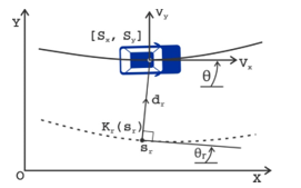
Figure 1. Vehicle model and reference curve

To facilitate the performance, in this paper we show the structure of the road as a system of roads defined by adjacent lanes of arbitrary shape and curvature. We assume and consider the i  to be a path defined by the left boundary  and the right boundary . Each such path is defined as a polyline and is a combination of all lanes at a given time interval ( ).

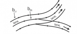
Figure 2. Road system model

The main idea when building a motion trajectory solution is to use a model predictive control (MPC) method, in which the set of constraints is constructed as logical propositions, including constraints on legal and ethical issues of traffic behavior. Based on the provisions of Vietnam traffic law, we perform logical clauses to introduce the constraint set in traffic as follows:

Rule 1: If the vehicle discovers obstacle ahead, it must slow down.

Rule 2: If it overtakes another vehicle, it must do so on the left side.

Rule 3: If it overtakes another vehicle on the right side, it must satisfy the condition that the vehicle ahead has given a signal to turn left or is turning left.

Rule 4: If it is traveling in an area where overtaking is prohibited or where the weather conditions do not ensure safe, it cannot overtake another vehicle.

Rule 5: If it changes lane or changes direction, it must give a turn signal.

Rule 6: If it changes direction, it must give way when detecting a vehicle ahead that is rudimentary vehicles and pedestrians.

Rule 7: If it moves in a residential area, the movement speed of the vehicle does not exceed 50 km/h and outside the residential area is 80 km/h.

Rule 8: If it performs changing lane and overtaking, it cannot do so continuously.

However, the issue of motion control decision depends on many situations, different states of the object types, and from which the vehicle’s motion trajectory is set appropriately. Therefore, for each class the object can be mapped to a single homotopy layer of trajectory. To describe these homotopy layers, we will also build with corresponding logical propositions. For example, the logical proposition of the homotopy class is described when meeting obstacles as follow:

Rule 9: Vehicle in motion, if it overtakes other vehicles, it must overtake on the left side or on the right side.

Rule 10: Vehicle in motion, if it avoids obstacle, it will overtake to the left or to the right of the obstacle and reduce its movement speed.

As we all know, the essence of predictive control is to use an explicit model of the object to calculate optimal variables controlled through optimization methods. Specifically, to control the prediction for an object, we need to perform the following steps: Building a predictive model, defining target functions and constraint conditions, and finally solving the optimal problem. At the same time a number of predetermined conditions such as communication between vehicles and future trajectories are determined [8, 9] during the construction of the trajectory of the motion plan.

With the idea of using the model predictive control and the first part of the proposed vehicle model with the state vector , control vector  as the basis for the research problem as follows:

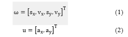
where  represent vertical and horizontal position, ,  are velocity and ,  are vehicle acceleration along the  axes of the vehicle in inertial frame.

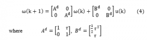
Then the dynamic model of the vehicle is represented with zero matrices of proper dimension, as follows:

In this problem, we make the assumption that the control vector  is a constant function at each time step . Therefore, the dynamical model of the vehicle is represented approximately with initial values including state vector and control vector  in time interval  as follows:

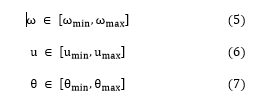
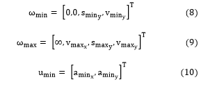
In order to achieve computational efficiency with the limitations of the vehicle’s dynamic system as well as the provisions about motion direction when overtaking obstacles on the road, it is necessary to consider the constraints on the state (.), the input control signal (.) and the motion direction of the vehicle (.) must meet the following conditions so that when the motion trajectory is built, it is feasible as follows:

In addition, in this problem we incorporate a set of constraints that are the provisions of the road traffic law. These provisions are considered as logical clauses and will perform the conversion into a set of linear inequalities with integer variables.

The transformation is done as follows: in the literals clause is represented as an indivisible statement with a linear expression on the state variables. The literals use logical operations like conjunction , disjunction , exclusive – OR , implication , equivalence , negation  to represent. At the same time, these literals will be represented as a binary variable  That only accepts 0 or 1 values, if a proposition is true then , otherwise it is false then .

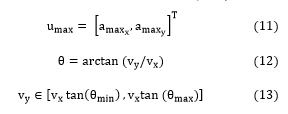
For example, to perform the constraint laws regulating about speed (Rule 1), travel speed (Rule 7) along with the structural constraints of the vehicle as follows: To ensure safety when participating in traffic then at position  from the starting position, will limit the vehicle movement speed to  (Figure 3), there will be 3 literals defined ,  and , and the logical clauses expressed at any point in the segment are .

Or we represent it after assigning a binary variable  with ,  as follows:

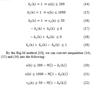
where  is a positive constant with great value. In this problem, we choose

Let  be the number of time steps in the prediction horizon with  be the time interval,  and  are state vectors, control trajectory vectors in the given time horizon,  is the reference trajectory of the vehicle, which may depend on time, status, or traffic law.

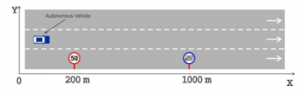
Figure 3. Speed limit ramp

To determine the objective function for this solution, we will introduce a new value vector variable  and , where  is a collection of all the binary variable results from the rebuilding the provisions of law on road traffic into linear inequalities and  is the reference trajectory for the binary variables where we can make options on some binary states.

Thus, at time , the optimal problem of the model predictive control with the objective function can be written as follows:

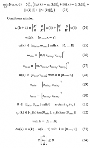
where the matrices C, D, Q, R, S and W are positive weight matrices of proper dimension, the final constraint (34) is the set of all provisions of road traffic law into linear inequality is represented in matrices.

The objective function (23) will be quadratic if the values of  and  are independent or linearly dependent on other variables. Therefore, solving this optimization problem will result in the global optimal trajectory being used so that it will then move to the controller at a lower level in tracking this trajectory.

Thus, given this optimal problem with the correlation and integration issues between vehicle dynamics and the provisions of the road traffic law, this solution can be used to effectively handle during the motion planning process with different situations during travelling. In order to achieve the optimal motion trajectory, it is necessary to process the cost function to a minimum and at the same time constraints including vehicle dynamics constraints and rules of participating in traffic after converting into logical constraints, it should be separated.

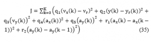
From the idea raised for this problem and in order to evaluate the effectiveness of the solution for the specific operating environment of the vehicle, the cost function is designed to optimize operational control with the initial condition that the vehicle velocity is constant and the horizontal deviation will change over time during the travel distance. Therefore, the expression  in the optimal problem (23) will not be considered, so the cost function built in this study is given as follows:

3. Experimental assessment

In order to ensure the reliability, objectivity and effectiveness of the solution, we have conducted simulations with different scenarios such as assessments on the roads with speed limit signs, determining the motion trajectory of the vehicle when there is an obstacle or a motion trajectory of the vehicle when overtaking in the same direction.

In the process of checking and evaluating the given solution, we conduct empirical simulation of processes in the Matlap environment. In which the calculation (using the SI measurement system) with the sampling period  and the predictive horizon . During the simulation, vehicles with recorded trajectory will be considered vehicles ahead and the autonomous vehicle will be behind these vehicles. The parameters used in the experimental process are given as follows:

The location of the experimental vehicle is in the right lane with the original position at the coordinates (0, 0), the original and constant speed during the experiment of the vehicle is . The trajectory switches to the I/O controller with a simulation time of .

Scenario 1: In this scenario, the autonomous vehicle will move into a road with limited speed (Figure 4). At the beginning, the traveling speed of autonomous vehicles is stable . When entering the prescribed speed range, with the input values ​​and constraints for the control system will be able to make the vehicle’s movement speed change. The control system will perform the braking operation to reduce vehicle speed to a safe limit with restrictions on road traffic rules. With such a driver assistance process, it shows the advantages of controlling the longitudinal force, horizontal force and acceleration the vehicle, as well as implementing the vehicle’s movement plan to be complete when coming to the road systematic motion velocity regulation.

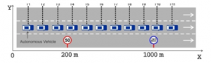
Figure 4. The vehicle moves over the speed limit segment

During the simulation process, with the parameters shown, the construction of constraints according to Rule 7 is carried out as follows:

When the vehicle moves into position T4 , it will limit the movement speed of the vehicle is , there will be 3 literals defined ,  and , and the logical propositional represented at all times in the segment is  . The constraints set is constructed to include:

where M is a positive constant with great value. In this simulation, we choose

The simulation results show that the movement speed of the vehicle from position T4 to position T10 according to the vehicle’s planning of movement decreases below the speed of , so the motion controller has been effectively applied.

Scenario 2: In this scenario, the autonomous vehicle will move in the same lane with other vehicles and the autonomous vehicle will perform the right overtaking for the vehicle ahead (Figure 5). At the beginning, the autonomous vehicle and other vehicles are in one lane with the distance from autonomous vehicle to the vehicles ahead is 30m, the initial speed of the vehicles ahead is 30km/h and of autonomous vehicles is 60km/h.

At the time of T3, the vehicle in front of the vehicle moved at a constant speed, in this situation, the vehicle would either self-drive or reduce the speed of  or perform an overtaking operation or an accident will occur. During the simulation, we choose to overtake and to ensure that overtaking does not violate road traffic rules, autonomous vehicle must perform overtaking in accordance with Rule 2.

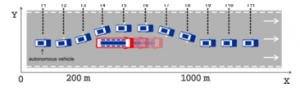
Figure 5. Autonomous vehicle passing to the right of the vehicle ahead

To set the control input values, we will describe the vehicles in front surrounded by rectangles. Each different object will have rectangles of different sizes and positions respectively. In this simulation, the position of the vehicle in front is   and the rectangle surrounding the vehicle in front is   and the width of . The rectangle around the vehicle in front of  is defined in the coordinate system as  with .

Thus, the constraint set is constructed to avoid collisions by overtaking on the right side as follows:

or represented by the following inequalities:

where M is a positive constant with great value. In this simulation, we choose

The simulation results show that the moving speed of the vehicle from position T1 to position T11 according to the movement plan of the vehicle is almost unchanged , but the steering angle of the vehicle begins to change from position T2 to position T5 is , from position T6 to position T8, it decreases to  and from position T9 the steering angle . The change of steering angle can be explained as follows, from position T2 the vehicle begins to move the steering angle to the right from the original movement direction to avoid collision and proceed to overtake to the right side of the object. After overtaking the object, at the position of T6, the autonomous vehicle will move back to the left side to return e original direction of movement. From position T9, the autonomous vehicle has passed the object and adjusted the angle back to the original to return to the original motion trajectories.

Scenario 3: In this scenario, the autonomous vehicle will move through an intersection, no traffic lights, no priority roads and no priority vehicles (Figure 6). As illustrated in Figure 6, there will be the following situations: i) the autonomous vehicle crosses the intersection before other vehicles, ii) the autonomous vehicle overtakes the intersection after vehicle 01 and before vehicle 03, iii) the autonomous vehicle overtakes the intersection after vehicle 03 and before vehicle 01, iv) the autonomous vehicle crosses the intersection after all the vehicles. In these situations, because the direction of vehicle 02 does not affect the movement of the autonomous vehicle, the presence of vehicle 2 is not considered in these situations.

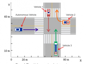
Figure 6. The vehicle moves into the intersection

To perform this simulation, we need to understand some rules when traveling through the intersection according to the provisions of Vietnam’s road traffic law as follows: Is there a vehicle to the intersection?, is there a priority vehicle or not?, is there a priority path?

Vehicles are considered to enter the intersection when the front wheel has crossed the white line of the zebra crossing. In any circumstance, a vehicle that enters the intersection is given priority to go first.

For priority vehicles, the order of vehicles prioritized includes fire engines, military vehicles, police vehicles, ambulances, and other priority vehicles such as dyke protection vehicles, convoy of vehicles with police leading the way, vehicles on missions to overcome natural disasters, epidemics or vehicles on emergency duty as prescribed by law. Priority vehicles will be moved in front of other vehicles, meaning that the non-priority vehicles must give way to the priority vehicles in traffic.

For priority roads, vehicles located on non-priority roads must give way to vehicles on priority roads and should be based on the “intersection with priority roads” signs.

If there is no vehicle in the direction, the following shall be prescribed: at the intersection, priority shall be given to the vehicle that there is no vehicle to the right hand direction, at the roundabout, the priority shall belong to the vehicle that there is no vehicle to the left hand direction. Finally, for the priority turning direction, it is regulated that the vehicle that turns right goes first, then the vehicle goes straight and finally the vehicle turns left.

In this simulation scenario, the simulated vehicles are running at a speed of 50km/h, the position of the vehicles considered in the coordinates respectively is the autonomous vehicle at position (10,45), vehicle 01 at position (45.65), vehicle 02 at position (80.55) and vehicle 03 at position (65.10), the center of the intersection is at (60.55).

The problem of this simulation is performed as follows: Let the file  be the part of the autonomous vehicle and  is the path of other vehicles in the intersection area. To avoid collisions between vehicles, only one vehicle is at any time in the intersection. Therefore, if ,  with , ie if the autonomous vehicle is already in the intersection, other vehicles cannot move into the intersection to avoid collisions at the intersection, where the values of  and  are symbols of the starting time and the last exit time of the vehicle while in the intersection .

When planning movement for an autonomous vehicle, we need to monitor whether other vehicles have entered the intersection area or not. First we will calculate the values ​​of   with   is assumed to be continuous increase and   with   is assumed to be a continuous decrease of other vehicles, where  is a time function to travel over a distance of path , with the current velocity  and acceleration of vehicle unchanged . In case the vehicle cannot travel the entire distance  in a finite time, this time value will be determined as , the values ​​  and  are introduced to replace the constant acceleration value in order to determine the error limit during the evaluation of the motion of other vehicles.

The prediction horizon  and   of other means are calculated as follows:

where  is the number of time steps in the prediction horizon.

Thus, with  being the prediction horizon of the autonomous vehicle, the constraint set is built to avoid collisions when the autonomous vehicle moves through intersections written with the following cases:

1. If , it means the autonomous vehicle will have to cross the intersection before another vehicle moves into the intersection area, or the autonomous vehicle must stay outside the intersection until another vehicle leaves the intersection area, then the constraint set will be:
2. If , it means the autonomous vehicle will have to go through the intersection before another vehicle moves into the intersection area, or the autonomous vehicle must be outside the intersection to the end of the prediction horizon, , then the constraint set will be
3. If , it means the autonomous vehicle will have to stay outside the intersection until other vehicles have moved through the intersection, no constraints are considered at this time.

The simulation results show that the speed of the autonomous vehicle decreases when preparing to enter the intersection area and then returns to the original speed, while moving through the intersection after all other vehicles. For a comparative basis, we tried to change the position of the autonomous vehicle at the new positions (45.45). Observing the process we realized that the autonomous vehicle moved through the intersection behind vehicle 1 and 2, but in front of vehicle 3 and the speed of vehicle 3 decreases when entering the intersection to make way for the autonomous vehicles to pass.

4. Conclusions

This paper proposes a solution to create the optimal trajectory with a model predictive control approach and the constraint set built from road traffic law. This approach is suitable for complex environmental conditions because these constraints can arise from various aspects of motion planning that must comply with traffic rules.

The motion trajectory of the vehicle is created from this solution aiming to improve performance and enhance the ability to avoid obstacles but still ensure optimal global trajectory. Simulation results with situations such as avoiding obstacles, passing other vehicles, moving through intersections … have shown that this solution achieves the set goal of improving calculation efficiency and handling of uncertainty in the perceptual data of the environment. However, with the use of a second-order linear vehicle model to create motion trajectories, this solution is only advantageous when applied in the case of the autonomous vehicle moving on a straight path. For large curves, the current model built may not be accurate.

Evaluating of safety conditions, the proposed solution has been effective. This motion planning method has created an optimal trajectory that allows an autonomous vehicle to drive along the road and avoid obstacles safely. To improve the efficiency of calculations and consider the uncertainty of perceptual data and positioning on the general trajectory, the performance of this proposed solution depends on the probabilistic model of the system to create adaptive fields. Therefore, probabilistic analysis and the representation of a driving situation need to be more integrated into actual vehicle application.

In the future, in order to increase the reliability of this solution, the settings that have been experimented by simulation will be transferred to the real environment with experimental vehicles equipped with sensors, and when experimenting on reality, a number of factors to analyze the stability of the system will be added so that the behavior of traffic participants is more accurately forecasted. Extensive implementation of this driver-assisted solution for semi-autonomous or fully autonomous vehicles in vehicle control systems will be able to minimize the amount of damage and create a safe movement plan for the future.

1. Bevan, Gollee and O’Reilly, Trajectory generation for road vehicle obstacle avoidance using convex optimization, Proc IMechE Part D: J Automobile Engineering, pp.455–473, 2010. DOI: 10.1243/09544070JAUTO1204.
2.  Jo K, Kim J, Kim D et al, Development of autonomous car – Part I: distributed system architecture and development process, IEEE Trans Ind Electron, pp.7131–7140, 2014. DOI: 10.1109/TIE.2014.2321342
3.  Zhang D, Li K and Wang J, Radar-based target identification and tracking on a curved road, Proc IMechE Part D: J Automobile Engineering, pp.39–47, 2012. DOI: 10.1177/0954407011414462
4.  A. Houenou, P. Bonnifait, V. Cherfaoui et al, “Vehicle trajectory prediction based on motion model and maneuver recognition.” in Proc of the IEEE Conference on Intelligent Robots and Systems, pp. 4363 – 4369, 2013. DOI: 10.1109/IROS.2013.6696982
5.  Fraichard and Howard, Iterative motion planning and safety issue, In: Eskandarian A Handbook of intelligent vehicles. London: Springer, pp. 1433–1458, 2012. DOI: 10.1007/978-0-85729-085-4_55
6.  M. Werling, S. Kammel, J. Ziegler et al, “Optimal trajectories for time-critical street scenarios using discretized terminal manifolds.” The International Journal of Robotics Research, vol. 31, no. 3, pp. 346–359. 2012. DOI: 10.1177/0278364911423042
7. S. J. Anderson, S. C. Peters, T. E. Pilutti et al, “An optimal-control-based framework for trajectory planning, threat assessment, and semi-autonomous control of passenger vehicles in hazard avoidance scenarios.” Transactions on International Journal of Vehicle Autonomous Systems, vol. 8, no. 2/3/4, pp. 190 – 216, 2010. DOI: 10.1504/IJVAS.2010.035796
8.  M. Althoff and J. M. Dolan, “Online verification of automated road vehicles using reachability analysis”, IEEE Trans. on Robotics, vol. 30, no. 4, pp. 903 – 918, 2014. DOI: 10.1109/TRO.2014.2312453
9.  M. Althoff, D. Heß, F. Gambert, “Road occupancy prediction of traffic participants.” in Proc. of IEEE Conference on Intelligent Transportation Systems, pp. 99–105, 2013. DOI: 10.1109/ITSC.2013.6728217
10.  Richard W. Cottle, Mukund N. Thapa, Linear and Nonlinear Optimization (2nd ed.), International Series in Operations Research & 15Management Science, 2017, DOI: 10.1007/978-1-4939-7055-1.

(Click Here)

(Click Here)