1. Introduction

The classical methods in statistical inference, such as confidence intervals estimation, are widely used by researchers in many disciplines. In the usage of the confidence intervals, the assumptions such as normality and no presence of outliers must be satisfied. Unfortunately, these assumptions are rarely met when analyzing real data in many fields of research such as engineering, data science, medical, public health, biological etc. The confidence intervals provide better information that of point estimator about the population characteristic of interest. The performance of confidence intervals for the appearance of outliers and under non-normal assumption have drawn much attention among the researchers. A variety of procedures are exist in the literature to construct the confidence interval (CI) for the population mean (μ), though the classical normal confidence interval is widely used. Nevertheless, the classical normal confidence interval requires normality assumption which most of the data do not follow in reality, particularly in presence of outliers. Thus, the robust estimators, which are less affected from non-normality assumption or outliers, are introduced in this paper in order to overcome such situations.

  Student’s-t confidence interval for the population mean (µ) has been used for a long period of time.  It has an approximate      (1- α) coverage probability (CP) under the condition of positively skewed distribution or there are some outliers in the data. However, this coverage probability may be improved by developing different confidence interval methods. The bootstrap confidence interval [1] is another method to construct the confidence intervals for the population mean which many researchers are suggested. The construction of this confidence interval has concerned about resampling technique which is complicated procedures and it has a good performance in theoretical coverage probability, but it tend to be erratic in actual practice depend on the distribution of the bootstrap estimator. Further, this method hard to implement in practices because it is not easy to compute without the statistical programming [2], while the two robust confidence intervals that are proposed in this paper are easy to implement in practices. The two robust confidence intervals for the population mean (μ) are proposed based on robust location and scale estimators in the case of non-normal distributions and contamination of outliers in the data set. We compare the performance of proposed robust methods with  that of the classical Student’s confidence interval using coverage probability and average width for non-normal distributions (symmetric and skewed ones) via a Monte-Carlo simulation study. For more on robust estimators, we refer  [3], Abu-Shawiesh [4, 5]  among others.

The organization for the remaining of this paper are the following: Section 2 is represented the proposed confidence intervals. A Monte-Carlo simulation study has been conducted in section 3.  Two real-life data are analyzed for the implementation of several methods in Section 4. Section 5 provides some concluding remarks.

2. Proposed Interval Estimators

2.1. The Classical Confidence Intervals for the Population Mean

A random sample X₁, X₂, …, X_n  of size n is taken from the population that is normally distributed with mean (μ) and variance (σ²). Then, the (1 – α) 100% classical confidence interval (CI) for the population mean (μ), for known σ is defined by (1).

where is the ( )^th percentile of the standard normal distribution. However, in real life, it is unlikely that the population standard deviation (σ) is known, and then an estimate of σ is needed. To do that, we can use the sample standard deviation (S) instead of the unknown population standard deviation (σ) and apply the normal distribution to construct the      (1 – α) 100% classical confidence interval (CI) for the population mean (μ) which is given by (2).

Since the classical confidence interval requires the normality assumption, it is unlikely that it will give good results when data are not normal. Therefore, we suggested two robust confidence interval estimators, namely, the median interquartile range confidence interval (MDIQR-CI) and the trimean interquartile range confidence interval (TRIQR-CI) and they are discussed as follows:

2.2. The Robust Confidence Intervals

We propose two robust modifications of the classical normal interval estimator for the population mean (μ) in the case of non-normal distributions and presence of outliers. They are simple adjustments based on robust estimators for location and scale parameters. The proposed robust confidence intervals for the population mean (μ) are introduced in these subsections:

2.2.1. The Median Interquartile Range Confidence Interval    

In this confidence interval (MDIQR-CI), we estimate the population mean (μ) by the sample median (MD) and the population standard deviation (σ) by   interquartile range (IQR). The standard error of the sample median (MD), that is , is used in the construction of this interval estimator. Thus, the (1 – α) 100% MDIQR-CI confidence interval for the population mean (μ) is given by (3).

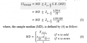
2.2.2. The Trimean Interquartile Range Confidence Interval

In this confidence interval (TRIQR-CI), we estimate the population mean (μ) by the sample trimean (TR) and the population standard deviation (σ) by   interquartile range (IQR). The standard error of the sample trimean (TR), that is , is used in the construction of this confidence interval. Then, the (1 – α) 100% TRIQR-CI confidence interval for the population mean (μ) is given by (5).

is the sample trimean and Q₁, Q₂ and Q₃ are the first, second (sample median) and third quartiles, respectively [6].

3.  The Simulation Study

A simulation study has been conducted to compare the performance of three interval estimators. The simulation method is one of techniques to implement for a theoretical performance comparison and the results of the study are usually very close to the ones of the exact case when using a large number of iterations. In order to make the comparisons among three confidence intervals, two performance criteria–the coverage probability (CP) and the average width (AW)–of the confidence intervals are considered. If the confidence interval that is compared among the three confidence intervals has a smaller width, it indicates this confidence interval is a better method for the same level of the coverage probability. For a higher coverage probability, the confidence interval indicates a better method when the widths are the same level.  We used SAS version 9.4 programming to conduct this simulation study. We consider the widely used 95% confidence intervals for this simulation.  We consider in equals to 10, 20, 30, 40, 50 and 100 were generated 100,000 times for each situation. For each data set of the samples, the common 95% confidence intervals were constructed for the three methods. The coverage probability (CP) and the average width (AW) of the confidence intervals are found by using respectively:

To compare the performance of the interval estimators, the same types of distributions are used as in [7–9]; symmetric, skewed and contaminated normal ones. So, there are three cases for the simulated observations as follows:

Case (a): Skewed Distributions

In the skewed distribution cases, we will simulate observations from the gamma distribution, given by (8):

where α and β are   the shape and scale parameters respectively. The mean of the distribution is given by and the variance of the distribution is given by . Without loss of generality, β is set to unity and if α increases then the gamma distribution will approach to the normal distribution. For this simulation study, we consider, α = 1, 2, 4, 8 and β =1.

Case (b): Symmetric Distributions

In the symmetric distribution cases, we will simulate observations from the student t-distribution, , where k is the numbers of degrees of freedom with probability density function ( ) given by (9):

where mean of the distribution is zero and the variance, . The t-distribution is one type of a symmetrical distribution and bell shaped around 0, but it has heavier tails than the normal distribution. Additionally, as the number of the degrees of freedom (k) increase, the t-distribution will approach to the normal distribution. For the simulation purposes, we will consider  = 4, 10, 30, 50.

Case (c): Contaminated Normal Distribution

In this case, we will simulate observations from mixture distribution that is called the contaminated normal distribution (CND) where artificial outliers are introduced in the data to assess the sensitivity of the three different interval estimators to the presence of outliers. The contaminated normal probability density function is given by (10):

where ) denote the normal PDF, (1 –  ) and  be the mixing probabilities, and the standard deviation of the wider component is defined as λ > 1. The main distribution of a data set is generated from the normal distribution  and slightly contaminated by a wider distribution. This paper determines  = 0.1, 0.2 and 0.3 which represents 10%, 20% and 30% “contamination” respectively, and assigns λ =   as the scale multipliers. In this section, we consider an uncontaminated standard normal distribution . The following six cases are constructed the PDF of the contaminated normal distribution (CND) as the linear combination of  and  densities as shown in (11) to (13), and the PDF of a contaminated normal distribution is the linear combination of   and   densities as shown in (14) to (16):

Case 1: A situation that comprises of 90% of simulated observations are sampled from  distribution and 10% from a normal distribution with mean and variance , , is generated. This will give approximately 10% artificial outliers.

Case 2: A situation that consists of 80% of simulated observations are sampled from the standard normal distribution, , and 20% from a normal distribution with mean and variance , , is generated. This will give approximately 20% artificial outliers.

Case 3: A situation that consists of 70% of simulated observations are sampled from the standard normal distribution, , and 30% from a normal distribution with mean and variance , , is generated. This will give approximately 30% artificial outliers.

 

Case 4: A situation that consists of 90% of simulated observations are sampled from the  distribution and 10% from a normal distribution with mean and variance , , is generated. This will give approximately 10% artificial outliers.

Case 5: A situation that consists of 80% of simulated observations are sampled from  distribution and 20% from a normal distribution with mean and variance , , is generated. This will give approximately 20% artificial outliers.

Case 6: A situation that consists of 70% of simulated observations are sampled from  distribution and 30% from a normal distribution with mean and variance , , is generated. This will give approximately 30% artificial outliers.

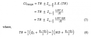
The simulation study results for all considered cases are presented in Table 1 to Table 4 and Figure 1 to Figure 4. The results in Table 1 and Figure 1 show the performances of skewed distribution cases that the observations are generated from gamma distribution with  equals 1, 2, 4, 8 and  equals 1. It is found that the coverage probabilities of the three confidence intervals tend to be lower than the nominal level (0.95) when the shape parameter equals 1, 2 and 4 for almost all sample sizes. When a shape parameter equals 8, the coverage probabilities of MDIQR and TRIQR confidence intervals are greater than the nominal level (0.95) for most of the sample sizes, whereas this of the classical confidence interval tends to be lower than the nominal level for all sample sizes. For all the shape and scale parameters of the gamma distribution, it is found that the classical interval estimator has the smallest average width of the confidence interval among the comparative confidence intervals for all sample sizes.

The simulated results in Table 2 and Figure 2 show the performances of symmetric distribution cases that the observations are generated from the Student’s t-distribution with DF   equals  4,  10,  30,  50.  It   is  observed   that  the   coverage

Table 1: Coverage probability (CP) and average width (AW) of the 95% CIs for gamma distributed data

PDF	n	Confidence Interval Methods
		Classical CI		MDIQR-CI		TRIQR-CI
		CP	AW	CP	AW	CP	AW
	10	0.8695	1.15	0.8485	1.70	0.8360	1.49
	20	0.9045	0.84	0.8251	1.21	0.8290	1.06
	30	0.9182	0.69	0.7697	0.98	0.7889	0.86
	40	0.9239	0.61	0.7162	0.85	0.7559	0.75
	50	0.9300	0.54	0.6558	0.76	0.7123	0.67
	100	0.9390	0.39	0.3796	0.54	0.5064	0.47
	10	0.8937	1.66	0.9125	2.64	0.8977	2.31
	20	0.9181	1.20	0.9143	1.89	0.9079	1.66
	30	0.9280	0.99	0.8943	1.54	0.8929	1.35
	40	0.9325	0.86	0.8752	1.34	0.8824	1.17
	50	0.9348	0.77	0.8521	1.20	0.8649	1.05
	100	0.9428	0.55	0.7152	0.85	0.7727	0.74
	10	0.9034	2.38	0.9409	3.91	0.9272	3.42
	20	0.9269	1.72	0.9520	2.80	0.9448	2.45
	30	0.9332	1.41	0.9453	2.29	0.9400	2.01
	40	0.9369	1.23	0.9394	1.99	0.9387	1.74
	50	0.9393	1.10	0.9306	1.78	0.9330	1.56
	100	0.9440	0.78	0.8789	1.26	0.8981	1.10
	10	0.9104	3.38	0.9526	5.65	0.9401	4.94
	20	0.9311	2.44	0.9685	4.06	0.9613	3.55
	30	0.9366	2.00	0.9671	3.32	0.9618	2.90
	40	0.9400	1.74	0.9659	2.88	0.9631	2.52
	50	0.9409	1.56	0.9624	2.58	0.9606	2.26
	100	0.9455	1.10	0.9453	1.83	0.9510	1.60

Table 2: Coverage probability (CP) and average width (AW) of the 95% CIs for t-distributed data

PDF	n	Confidence Interval Methods
		Classical CI		MDIQR-CI		TRIQR-CI
		CP	AW	CP	AW	CP	AW
	10	0.9259	1.63	0.9712	2.33	0.9602	2.04
	20	0.9399	1.18	0.9856	1.65	0.9792	1.44
	30	0.9433	0.98	0.9878	1.33	0.9815	1.17
	40	0.9453	0.85	0.9901	1.16	0.9856	1.01
	50	0.9474	0.77	0.9904	1.03	0.9862	0.90
	100	0.9474	0.55	0.9921	0.73	0.9886	0.64
	10	0.9207	1.34	0.9676	2.15	0.9562	1.88
	20	0.9369	0.96	0.9835	1.53	0.9779	1.34
	30	0.9418	0.79	0.9859	1.25	0.9809	1.09
	40	0.9431	0.69	0.9885	1.08	0.9848	0.95
	50	0.9447	0.62	0.9892	0.97	0.9862	0.85
	100	0.9476	0.44	0.9912	0.69	0.9895	0.60
	10	0.9182	1.25	0.9665	2.08	0.9555	1.82
	20	0.9372	0.89	0.9838	1.49	0.9786	1.30
	30	0.9413	0.73	0.9860	1.22	0.9820	1.06
	40	0.9436	0.64	0.9880	1.06	0.9855	0.92
	50	0.9452	0.57	0.9888	0.94	0.9861	0.83
	100	0.9469	0.40	0.9902	0.67	0.9888	0.59
	10	0.9176	1.23	0.9663	2.06	0.9547	1.80
	20	0.9362	0.88	0.9832	1.48	0.9778	1.30
	30	0.9404	0.72	0.9851	1.21	0.9809	1.06
	40	0.9432	0.63	0.9878	1.05	0.9850	0.92
	50	0.9442	0.56	0.9887	0.94	0.9861	0.82
	100	0.9476	0.40	0.9905	0.67	0.9893	0.58

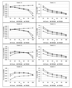
Figure 1: Coverage probabilities and average widths of the three confidence intervals for gamma distributed data

probabilities of the MDIQR and TRIQR interval estimators tend to be greater than 0.95, whereas this of the classical confidence interval tends to be lower than 0.95 for all sample sizes and all the numbers of DFs for the t-distribution. When considering the average width of interval estimators, it is found that the classical confidence interval has the smallest value among the comparative   interval estimators for all sample sizes and DFs.

The simulated results in Table 3 and Figure 3 demonstrate the performances of contaminated normal distribution cases that the observations are generated from the linear combination of   and   densities with 90%, 80% and 70% of observations are sampled from the N(0, 1) distribution and respectively of 10%, 20% and 30% are sampled from a N(0, 25) distribution. The simulation study shown that the coverage probabilities of the MDIQR and TRIQR interval estimators tend to be greater than 0.95, whereas this of the interval estimators is about 0.95 for all sample sizes and all percentages of the artificial outliers. For the case of linear combination of   and   densities, the TRIQR confidence interval has the smallest average width among the comparative interval estimators for all sample sizes and all percentages of the artificial outliers. That is, the 95% TRIQR interval estimator tends to have the best performance for both criteria–coverage probability and average width of the confidence interval–in this case.

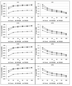
Figure 2: Coverage probabilities and average widths of the three confidence intervals for t-distributed data

Table 3: Coverage probability (CP) and average width (AW) of the 95% CIs for contaminated normal distributed data as the linear combination of N(0, 1) and N(0, 5²) densities

CND	N	Confidence Interval Methods
		Classical CI		MDIQR-CI		TRIQR-CI
		CP	AW	CP	AW	CP	AW
	10	0.9443	2.06	0.9682	2.27	0.9566	1.98
	20	0.9547	1.52	0.9845	1.62	0.9784	1.42
	30	0.9523	1.27	0.9859	1.33	0.9812	1.16
	40	0.9528	1.11	0.9888	1.15	0.9854	1.01
	50	0.9512	1.00	0.9891	1.03	0.9855	0.90
	100	0.9494	0.71	0.9912	0.73	0.9894	0.64
	10	0.9509	2.75	0.9725	2.57	0.9610	2.25
	20	0.9495	2.02	0.9869	1.83	0.9806	1.60
	30	0.9484	1.67	0.9880	1.49	0.9821	1.30
	40	0.9478	1.46	0.9903	1.29	0.9856	1.13
	50	0.9483	1.31	0.9905	1.15	0.9857	1.01
	100	0.9479	0.93	0.9925	0.81	0.9892	0.71
	10	0.9435	3.32	0.9780	3.11	0.9685	2.73
	20	0.9433	2.42	0.9896	2.12	0.9833	1.86
	30	0.9436	2.00	0.9907	1.70	0.9840	1.49
	40	0.9443	1.74	0.9920	1.47	0.9861	1.29
	50	0.9464	1.57	0.9927	1.31	0.9865	1.15
	100	0.9482	1.11	0.9938	0.92	0.9886	0 .81

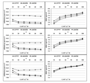
Figure 3: Coverage probabilities and average widths of the three confidence intervals for contaminated normal distributed data as the linear combination      of N(0, 1) and N(0, 5²) densities

The simulated results in Table 4 and Figure 4 show the performances of contaminated normal distribution cases that the observations are generated from the linear combination of   and   densities with 90%, 80% and 70% of observations are sampled from the N(0,1) distribution and respectively of 10%, 20% and 30% are sampled from a N(0, 100) distribution. In this case, the TRIQR confidence interval performs the best efficiency among the three interval estimators for all sample sizes and all percentages of the artificial outliers because the coverage probability of this interval estimator is greater than 0.95 and it has the smallest average width of interval estimator. In addition, the efficiency of MDIQR confidence interval is similar to this of TRIQR interval estimator. In this case, it is found that the classical interval estimators is not robust to outliers–that is, it has the highest average width of interval estimator and the coverage probability of it is smaller than the two proposed robust methods for almost all sample size, especially for a large percentage of outliers.

Table 4: Coverage probability (CP) and average width (AW) of the 95% CIs for contaminated normal distributed data as the linear combination of N(0, 1) and N(0, 10²) densities

CND	n	Confidence Interval Methods
		Classical CI		MDIQR-CI		TMIQR-CI
		CP	AW	CP	AW	CP	AW
	10	0.9665	3.46	0.9693	2.30	0.9576	2.02
	20	0.9766	2.63	0.9850	1.65	0.9786	1.44
	30	0.9704	2.21	0.9865	1.35	0.9814	1.18
	40	0.9650	1.95	0.9891	1.17	0.9854	1.02
	50	0.9604	1.76	0.9894	1.04	0.9856	0.91
	100	0.9520	1.27	0.9915	0.74	0.9894	0.65
	10	0.9775	5.08	0.9746	2.68	0.9629	2.34
	20	0.9609	3.78	0.9885	1.90	0.9818	1.67
	30	0.9524	3.14	0.9890	1.54	0.9828	1.35
	40	0.9497	2.75	0.9913	1.33	0.9858	1.17
	50	0.9498	2.47	0.9911	1.19	0.9859	1.04
	100	0.9493	1.77	0.9931	0.84	0.9891	0.74
	10	0.9633	6.36	0.9832	3.85	0.9752	3.37
	20	0.9457	4.66	0.9930	2.39	0.9876	2.09
	30	0.9452	3.86	0.9927	1.84	0.9860	1.61
	40	0.9454	3.36	0.9942	1.58	0.9876	1.39
	50	0.9471	3.02	0.9941	1.40	0.9873	1.23
	100	0.9486	2.15	0.9951	0.98	0.9886	0.86

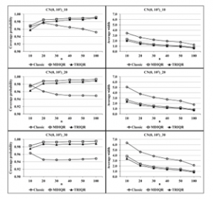
Figure 4: Coverage probabilities and average widths of the three confidence intervals for contaminated normal distributed data as the linear combination      of N(0, 1) and N(0, 10²) densities

Table 5: Melting points of beeswax data

No.		No.		No.		No.
1	63.78	16	63.92	31	64.42	46	64.12
2	63.83	17	63.86	32	63.50	47	63.03
3	63.88	18	63.13	33	63.84	48	63.66
4	63.78	19	63.08	34	64.21	49	63.34
5	63.50	20	63.30	35	64.40	50	63.34
6	63.41	21	63.51	36	62.85	51	63.56
7	63.45	22	63.56	37	63.27	52	63.92
8	63.63	23	63.93	38	63.36	53	63.68
9	63.36	24	63.69	39	64.27	54	63.60
10	63.92	25	63.40	40	64.24	55	63.50
11	63.30	26	63.83	41	63.61	56	63.92
12	63.60	27	63.51	42	63.31	57	63.39
13	63.58	28	63.43	43	63.10	58	63.53
14	63.27	29	63.43	44	63.86	59	63.13
15	63.36	30	63.05	45	63.50

4. Application with Real Data

 We consider two real-life examples from normal and non-normal distributions to illustrate the findings of the paper in this section.

4.1. Example 1: Melting Points of Beeswax Data

The data of this example is considered from [10] (cited in [11]), p.378) and introduced by [12].  Table 5 provides data representing the melting points (^oC) of beeswax obtained from 59 sources.

The statistical summary of the melting points (^oC) of beeswax data was calculated and given below in Table 6.

Table 6: Statistical summary for the melting points (^oC) of beeswax data

Statistics	Abbreviations	Values
Sample Mean		63.589
Sample Median	MD	63.530
Sample Trimean	TR	63.564
Sample Standard Deviation	S	0.347
Inter-Quartile Range	IQR	0.475

According to [12], it is known that the population mean of the melting point of beeswax ( ) is about  ^oC. The histogram, density plot, Boxplot and normal Q-Q plot are displayed in Figure 5. As can be observed, a goodness-of-fit test for normality assumption by using the Kolmogorov-Smirnov (K-S) statistical test provides a p-value is greater than a = 0.05 (KS = 0.086, p-value > 0.150), we conclude that the data are met a normal distribution assumption. The plots in Figure 5 are consistent with the above conclusion.

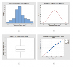
Figure 5: Plots for the melting points (^oC) of beeswax data

The 95% interval estimator of µ and the corresponding widths for the proposed intervals are given below in Table 7.

Table 7: The 95% CIs for the population mean ( ) of the melting points (^oC) of beeswax data

Methods	Confidence Interval Limits		Widths
	Lower Limit	Upper Limit
Classical	63.500	63.678	0.178
MDIQR	63.378	63.682	0.304
TRIQR	63.431	63.697	0.266

It is observed from Table 7 that all the interval estimators include the true population mean ( ). The classical interval estimator has the shortest interval width followed by CI_TRIQR and CI_MDIQR, so both the classical and proposed interval estimators did well. Hence, these results are consistent with the simulation study.

4.2. Example 2: Urinary Tract Infections (???) Data

The data of this example represent the duration of male patient urinary tract infections (????) in days and presented in Table 8. It was considered by various researchers, among them, [13–15] are notable. The summary statistics of the urinary tract infections (????) data are displayed in Table 9. The histogram, density plot, Box-plot and normal Q-Q plot are given in Figure 6. As it can be observed, the Kolmogorov-Smirnov (K-S) statistical test provides a p-value less than a = 0.01 (KS = 0.212, p-value < 0.010), which indicates that the data do not follow normal distribution. The plots in Figure 6 supported the above conclusion. It is noted from   Santiago and Smith (2013) that the data are well fitted to an exponential distribution with a mean time of µ = 0.2100 days.

Table 8: Urinary tract infection (UTI) data

No.		No.		No.
1	0.57014	19	0.12014	37	0.27083
2	0.07431	20	0.11458	38	0.04514
3	0.15278	21	0.00347	39	0.13542
4	0.14583	22	0.12014	40	0.08681
5	0.13889	23	0.04861	41	0.40347
6	0.14931	24	0.02778	42	0.12639
7	0.03333	25	0.32639	43	0.18403
8	0.08681	26	0.64931	44	0.70833
9	0.33681	27	0.14931	45	0.15625
10	0.03819	28	0.01389	46	0.24653
11	0.24653	29	0.03819	47	0.04514
12	0.29514	30	0.46806	48	0.01736
13	0.11944	31	0.22222	49	1.08889
14	0.05208	32	0.29514	50	0.05208
15	0.12500	33	0.53472	51	0.02778
16	0.25000	34	0.15139	52	0.03472
17	0.40069	35	0.52569	53	0.23611
18	0.02500	36	0.07986	54	0.35972

Table 9: Statistical summary for the urinary tract infections (????) data

Statistics	Abbreviations	Values
Sample Mean		0.2103
Sample Median	MD	0.1424
Sample Trimean	TR	0.1580
Sample Standard Deviation	S	0.2119
Inter-Quartile Range	IQR	0.2431

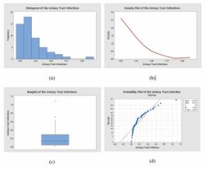
Figure 6: Plots for the urinary tract infections (????) data

The 95% interval estimator of µ and the corresponding widths for all proposed interval estimators are given below in Table 10.

Table 10: The 95% CIs for the population mean ( ) of the urinary tract infections (????) data

Methods Confidence Interval Limits Widths Lower Limit Upper Limit Classical 0.1538 0.2668 0.1130 MDIQR 0.0612 0.2236 0.1624 TRIQR 0.0869 0.2291 0.1422

It is observed from Table 10 that all interval estimator capture the true population mean ( ). The classical interval estimator has the shortest width followed by CI_TRIQR and CI_MDIQR, so both the classical and proposed interval estimators performed well. These results are consistent with the simulation study.

5. Some Concluding Remarks

For estimation of the population mean (μ), two robust interval estimators, namely, the median interquartile range (MDIQR-CI) and the trimean interquartile range (TRIQR-CI) are proposed in this paper. The simulation study evident that both criteria–coverage probability (CP) and average width (AW)–of the proposed robust interval estimators tend to have a good performance when observations are sampled from the contaminated normal distribution, especially for the high percentage of outliers and the main distribution is contaminated with the wider distribution. However, when observations are sampled from non-normal distributions, gamma and t-distributions, the classical confidence interval tends to have the best performance for the average width criterion, whereas the coverage probability of this tends to be smaller than those of the proposed robust interval estimators. Two data sets are analyzed to illustrate the performance of the interval estimators, which supported the simulation study. Finally, the proposed robust interval estimators are easy to compute, not computer intensive and promising, so that they can be recommended for the practitioners when these compare with the bootstrap confidence interval that suggested by [1]. As mention in the introduction section that bootstrap confidence interval complicates to implement in practices because it is not easy to compute without the statistical programming [2].

Conflict of Interest

The authors declare no conflict of interest.

Acknowledgment

Authors are thankful to anonymous referees and editor for their valuable comments and suggestions, which certainly improved the quality and presentation of the paper. Author, B. M. Golam Kibria wants to dedicate this paper to his most favorite teacher and guardian, late Prof. A. B. M. Abdus Sobhan Miah, Department of Statistics, Jahangirnagar University for his wisdom, constant inspiration during student life and affection that motivated him to achieve this present position.

1. B. Efron, R. J. Tibshirani, An Introduction to the Bootstrap, Chapman and Hall, 1993.
2. J. Carpenter, J. Bithell, “Bootstrap confidence intervals: when, which, what A practical guide for medical statisticians” Stat. Med., 19(9), 1141–1164, 2000.
   https://doi.org/10.1002/(SICI)1097-0258(20000515)19:9<1141::AID-SIM479>3.0.CO;2-F
3. M. L. Tiku, A. D. Akkaya, Robust estimation and hypothesis testing, new age international (P) limited, 2004.
4. M. O. Abu-Shawiesh, “A simple robust control chart based on MAD” Math. Stat., 4(2), 102-107, 2008.
   doi:10.3844/jmssp.2008.102.107
5. H. W. Akyüz, H. Gamgam, A. Yalçınkaya “Interval estimation for the difference of two independent nonnormal population variances” GU. J. Sci., 30(3), 117-129, 2017.
6. H. F., Weisberg, Central Tendency and Variability. Sage University Paper, USA: Series on Quantitative Applications in the Social Sciences, 1992.
7. C. M. Borror, D. C. Montgomery, G. C. Runger, “Robustness of the EWMA control chart to non-normality”
   J. Qual. Technol., 31(3), 309–316, 1999. https://doi.org/10.1080/00224065.1999.11979929
8. Z. G. Stoumbos, M. R. Jr. Reynolds, “Robustness to non normality and autocorrelation of individual control charts” J. Stat. Comput. Sim., 66(2):145–187, 2000. doi: 10.1080/00949650008812019
9. M. O. Abu-Shawiesh, F. M. Al-Athari, H. F. Kittani “Confidence interval for the mean of a contaminated normal distribution” J. Appl. Sci., 9(15), 2835-2840,
   2009. doi: 10.3923/jas.2009.2835.2840
10. J. White, M. Riethof, I. Kushnir, “Estimation of microcrystalline wax in beeswax” J. Assoc. Off. Anal. Chem., 43(4), 781-790, 1960. https://doi.org/10.1093/jaoac/43.4.781
11. J. A. Rice, Mathematical Statistics and Data Analysis. California, Duxbury Press, 2007.
12. W. Panichkitkosolkul, “Confidence interval for the coefficient of variation in a normal distribution with a known population mean after a preliminary t test”. KMITL Sci. Tech. J., 15(1), 34 – 46, 2015.
13. E. Santiago, J. Smith, ”Control charts based on the exponential distribution: adapting runs rules for the t chart” Qual. Eng., 25(2), 85-96, 2013.
    https://doi.org/10.1080/08982112.2012.740646
14. M. Aslam, N. Khan, M. Azam, C. H. Jun, “Designing of a new monitoring t-chart using repetitive sampling” Inf. Sci, 269, 210-216, 2014.
    https://doi.org/10.1016/j.ins.2014.01.022
15. M. Azam, M. Aslam, M., C. H. Jun, “An EWMA control chart for the exponential distribution using repetitive sampling plan” Operations Research and Decisions, 27(2), 5-19, 2017. doi: 10.5277/ord170201

(Click Here)

(Click Here)