1. Introduction

The supervision applications provided to control system developers (in manufacturing production, robotics, logistics, vehicle traffic, communication networks or IT) make it possible to report the detection of a dysfunction or accidental shutdown of the system and locate its origin. The discrete event systems (DES) community has developed diagnostic methods that focus on the logical, dynamic or temporal sequence of failure events that cause this dysfunction. However, the criticality of some systems and their complexity require a method of the failure events prognosis, to report their occurrence in advance in order to avoid any damage caused by a failure.

The challenge is therefore to prevent the future occurrence of a failure event. However, which suitable modeling tool is required for this system? And knowing that more the complexity of the system increases, more its state of space increase. So, how to overcome this problem of combinatorial explosion? And what are the prognosis limits?

Several fault prognosis methods have been developed; some have adopted a stochastic approach [1] [2] [3] while others have chosen non-stochastic [4]-[6], one for state automaton or Petri Net. These approaches are interested in prediction of failure m-steps in advance, based on a stochastic process. However, their assessment is difficult and probabilistic information is not always realistic. Others propose a prognosis approach [7] that consists of giving occurrence rates of possible traces that end with a failure event. These approaches indicate the occurrence of a future failure event, but do not specify its occurrence date. The possible occurrence date of a failure event makes it possible to plan the intervention date to repair the system before a failure occurs and thus provides visibility into the future evolution status of the system.

The challenge of each group working on this topic is to predict perfectly the future reality. [8] introduces the notion of signature of a trace, which consists to use several formal systems devoted to the description of event signature and the recognition of behaviors, called chronic. This concept has been used in diagnostic work [9], [10] and is based on error detection, localization, evaluation, recognition and response. [11] proposed a method for calculating the execution time of a trace, but it is still diagnosis-oriented. The development of a new approach of the temporal prognosis requires a modeling tool that allows the time constraints of the system (temporal prognosis) while using labels (it involves predicting an event over time). An extension of the Petri nets offers this possibility. These Petri nets are called, the Temporal Labelled Petri net (TLPN for short).

The aim is to propose a correct control of a system subject to unforeseen failures. The existing studies use the logical order of failure events occurrences to make the prognosis. In this paper, we are not only interested in the logical order of events, but also in the date of their occurrence. We assume that the system accepts three possible operating modes (nominal, degraded, and failed one). The events occurrence allows the system to switch between these modes. The event occurrence dates allow the synchronization of state switching in the model. A delay occurrence of an event, for example, can be explained by a degradation of the system. Approach’s based only of a logic events occurrence cannot detect this delay. Hence the interest of a time-based prognosis approach.

Two contributions are proposed in this paper. The first one is concerned with the formal representation and the second one with the methodology of prognosis calculation. Indeed, the model is based on a TLPN. The association of events to temporal transitions will be presented. The evolution from one mode to another one will be represented by transitions firing. The firing of each transition depends on the occurrence of an event and corresponding occurrence date. The second contribution relates to the methodology of the prognosis. A prognoser is built from the TLPN model. It is an oriented state graph, which identifies all possible sequences namely those that end in a failure event. But before predicting a failure event, it is important to make sure that it is possible to do it. That’s why we introduced the prognosability property whose objective is to determine the sequences ending with a failure event. Such event is called prognosable, the goal is to predict the earliest date of failure event occurrence. To calculate the execution time of these sequences and optimize the number of possible states, the resolution of an inequalities system based on works of [11]-[13] is used. The idea is to find the set of minimum values solution of the inequalities system. These values will constitute the minimum time after which the occurrence of the failure event is sure.

The paper is organized as follows: the second section is devoted to the basic concepts of Petri Nets (PN). The third section introduces temporal PNs (according to Berthomieu [14]-[19] and Popova [11]-[13], [20]-[22]. The fourth section focuses on labelled PN. In the fifth section, we discuss time-labelled PN to verify the prognosis approach in the sixth section. Thus, in this last section, the formal approach of our proposal will be presented, with an algorithm for predicting a temporal failure event and a case study, with explanations.

2.       Preliminary

2.1.  Petri Nets (PN)

A PN structure is a 4-uplet given by:
P is a nonempty finite set of places {p_1,p_2,…p_n}.
T is a nonempty finite set of transitions {t,t_2,…t_m} with
P∩T=∅.
Pre is the backward incidence function that assigns to each couple (p,t) of places and transitions a non-negative integer. Pre:P×T →N, Pre (p, t) =  is the value of the arc weight arc from the place p to the transition t.

Post is the forward incidence function that assigns to each couple (t,p) of transitions and places a non-negative integer. Post:T×P →N, Post (p, t) =  is the value of the arc weight arc from the transition t to place p.

The initial marking m_0 is an application:
m_0 ∶ P → N, it is labeled as an initial global system state. A marked net system 〖R_m=<R,m〗_0> is a net R with an initial marking m_0. When the transition t is enabled, it then would be fired. From the marking m, the firing of the t leads to the new marking m^’ denoted by m[t > m^’.
The symbol •t_j denotes the set of all places p_i such that Pre(p_i, t_j)  0 and t_j^• the set of all places p_i such that post(p_i, t_j)  0. Analogously, •p_i denotes the set of all transitions t_j such that post(p_i, t_j) 0 and p_i^• the set of all transitions t_j such that Pre(p_i, t_j) 0.

2.2.  Temporal Petri Nets (TPN)

Temporal Petri Nets TPN are introduced in [5], then studied by [16], [20]-[26].

Post is the forward incidence function that assigns to each couple (t,p) of transitions and places a non-negative integer. Post:T×P →N, Post (p, t) =  is the value of the arc weight arc from the transition t to place p.

An enabled transition t can be fired at time τ if the time elapsed since the activation of t belongs to the interval I(t) [T_min, T_max].
If T_min=T_max = 0 (i.e., I(t) = [0, 0]) the transition t is called immediate otherwise it is called timed.

Thus, we can divide the set T of transitions into two subsets T^t and T^im [27] where T^t is the set of timed transitions and T^im is the set of immediate transitions with: T^t∩T^im=∅ and T^t∪T^im=T

The aim of this distinction is to determine the firing priorities of the transitions. Firing  transitions has a higher priority than firing  transitions.

2.2.1. Behavior, states and reachability relation

Definition 2:

According to [1], a state of a temporal net is a pair E = ( , I) in which  is a marking and the application I associates a firing temporal interval to each transition.

The initial state consists of the initial marking m_0 and the application I_0 which associates to each enabled transition its static firing temporal interval, E_0=(m_0,I_0), such that:

Transition t may fire iff it remains logically enabled for a time interval  included in [Tmin; Tmax].  is the amount of time that has elapsed since the transition t is enabled.
A transition t is enabled in a state

From E, the result of the t firing is as usual the new state E’ = (m’, I’) such that:
m’ = m + ∆t with ∆t = Post(•,t) – Pre(•,t)
For each transition t_k:
If t_k is not enabled by m’, then I’(t_k) = ∅ ;
If t_k is distinct from t, enabled by m, and not in conflict with t, then I’(t_k) = [max (0, min(I(t_k)) – ), max( I(t_k))- ]
Otherwise I’(t_k) = I(t_k)

According to [11], a state of an TPN is a pair E = ( , h) in which  is a place marking (noted p_marking) and h is a clock vector (of dimension equal to the number of network transitions) that corresponds to the transition markings (noted t_marking). Thus, the p_marking describes the situation of the places and t_marking that of the transitions. Such a pair (p_marking, t_marking) describes a TPN status.

Definition 3:

Let  be an TPN.

A p_marking in R_T is a function m: P  ℕ. A p_marking in TPN is also a marking in a untimed PN.
A t_marking in R_T is a function h: T  ℝ ∪ {$}
$ means that the transition is not enabled.
Definition 4:
Let R_T = <P,T,Pre,Post,〖 m〗_0,I> a TPN, m is a p_marking and h is a t_marking. The pair E = (m, h) is called a state in R_T if and only if:
m is a marking accessible in R.
∀t (t ∈T∧Pre(•,t) ≰m ⟶h(t)=$).
∀t (├ t ∈T∧Pre(•,t) ≤m ⟶h(t)∈R_0^+ ∧h(t) ≤max⁡(t) ┤) where max⁡(t) is the latest firing time of t.

Definition 4 shows that each transition t has a clock. If t is not enabled by the marking , the associated clock is not activated (sign $), If t is enabled by , the clock of t indicates the time elapsed since the last activation of t.

A transition t is firable from state E = (m; h) (noted E[t> ) if and only if Pre(•,t)≤m and h(t)  min(t); (3) where min⁡(t) is the earliest firing time of t. The firing of t leads R_T to a new state E’ = (m’, h’) (noted E[t>E’)
In general, each TPN has an infinite number of states, depending formulation of time.

The construction of the reachability graph of a such PN is then generally impossible. To reduce this state space and provide a finite representation of the reachability graph, two different methods are defined. [14] Introduces the notion of state classes and [11] provides a parametric description to reduce this state space without affecting network properties. This reduced report space is used to define the reachability graph of a TPN. Such a graph will provide a basis to predict failure events of the system.

2.2.2. Parametric state and parametric sequence

Let R_T be an arbitrary TPN. Either σ=t_1…t_n a firing sequence in R_T and either τ=τ_0 τ_1…τ_n a time sequence with τ_i∈R^(*+). Then there is at least one dated sequence σ(τ)=τ_0 t_1 τ_1 t_2…τ_(n-1) t_n τ_n of  in R_T called the timed sequence of  which leads the net from the initial state E_0 to a state E (noted E_0 [()>E) with E = (m, h).
Let us consider for example the following sequence leading the network from the initial state E_0 to a state E_n :
E_0 [2.0>E_0^’ [t_1>E_1 [2.3>E_1^'[t_2> …t_n>E_n [1,5>E_n^’
The switch from E_0 to E_1 is made in 2 time units after the firing of t_1.
In addition to this feasible sequence, it is obvious that there is an infinity of feasible sequences leading R_T from E_0 to E, which makes the reachability graph infinite. Instead of considering fixed numbers τ_i, a variable x_i is used to denote the time elapsed between firing the transition t_i and the transition t_(i+1) in . Thus instead of having an infinity of execution sequences between the states E_0 and E_n, we will study a single sequence that we will call parametric sequence σ(x)=x_0 t_1… x_(n-1) t_n x_n leading the network from the state E_0 to the state E_n with E_0 [x_0>E_0^’ [t_1>E_1 [x_1>E_1^'[t_2> …t_n>E_n [x_n>E_n^’.
Definition 5: Parametric state and parametric sequence
Let R_T = <P,T,Pre,Post,〖 m〗_0,I> an TPN, σ=t_1…t_n a firing sequence in R_T, σ(x)=x_0 t_1… x_(n-1) t_n x_n its feasible sequence and〖 B〗_σ the value of x. The condition for the values B(x_i ) results from the time intervals associated with transitions and are united into the set B_σ (5). Then, the parametric execution (σ(x),B_σ) of σ and the parametric state (E_σ,B_σ) in R_T are determined by:

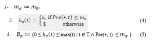
* Now, it is assumed that E_σ and B_σ are already defined for the sequence σ=t_1…t_n.
for σ=t_1…t_n t_(n+1)=γt_(n+1), and
σ(x)=x_0 t_1… x_(n-1) t_n x_n t_(n+1) x_(n+1) we put 1. m_σ≔m_γ+∆t_(n+1),

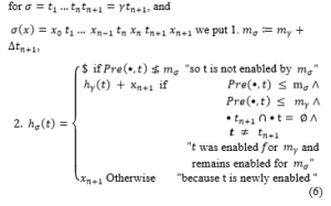
h_σ (t) is a sum of variables (6) (h_σ (t) is a parametric t_marking), it is a vector of linear functions: h_σ (t)= f(x) with x:= (x_0, … x|σ|)
B_σ is a set of conditions (7) (a system of inequalities)
Example:
Consider the temporal Petri Net

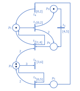
Figure 1: Model 1.

The POPOVA approach not only reduces the system’s state space (considering only the essential states) [12], but also determines the time required to reach each state. By using parametric states, it is not necessary to check all possible values of the clock, and the inequation system allows to determine the minimum values of their firing times. We will take advantage of this last remark to make the prognosis as soon as possible of a failure event.

2.3.  Labeled Petri net

In discrete event systems, partial observation often results in the addition of events or labels as sensor responses of the system.

Thus, a Labelled Petri Net (which we will note ) is a classic Petri net in which labels are associated to transitions.

Definition 6:

A Labelled Petri Net (LPN) is a net R_L=<P,T,Pre,Post,m_0,Σ,L> in which =<P,T,Pre,Post,m_0>, is a marked Petri net,  is the set of labels associated with transitions, L: T   ∪ {} is the transition labeling function associating a label (event) e ∈  ∪ {} to each transition t∈T, with  the empty event (or silent).
Thus: L (t) = e means that the label of the transition t is e.
Remark: Σ can be partitioned to Σ_o and Σ_uowith Σ_o is the set of observable events and Σ_uo is the set of unobservable events
In this paper we assume that the same label e ∈  can be associated with several transitions, i.e., two transitions t_i and t_j with t_i≠ t_j can be labelled with the same event e in a LPN.
Let * the set of all event trace  containing the label , the function of labeling transitions L can be extended to sequences: L : T*  * such that:

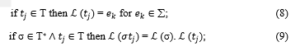
Moreover, if L (λ) =  then λ is the empty sequence.
Let σ a transition sequence and ω = L (σ) ∈ Σ^*. The labelled sequence lead to a language generated by the LPN R_L is L( R_L) = { ω ∈ Σ^* | (∃σ, m_0[σ>) L (σ) = ω}. Thus, m_1 [ω >m_2 means that ∃σ ∈ T∗, L (σ) = ω where ω=e_1 e_2…e_n that is, from m_1 and by firing σ, m_2 will be reached. m_2 can be noted m_σ. [27][28]. Note that the length of a sequence σ is greater than or equal to the corresponding word ω (i. e. |σ| ≥ | ω |). Indeed, if σ contains q transitions labeled by ε, then |σ|=q+| ω| Given the events sequence ω, the reverse labeling function L^(-1)(ω) is the whole { σ ∈ T* | L(σ) = ω }.
Example [27]:
Let the following alphabet Σ={e_1,e_2,e_3}, all transitions T={t_1,t_2,t_3,t_4} and the labelling function L such

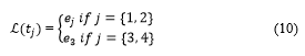
Let’s consider the set  = {e_1,e_3}, then L^(-1)() = {{t_1,t_3}, {t_1,t_4}}.

2.4.  Temporal labelled Petri net

In this paper, the aim is to provide a prognosis of the occurrence date a failed event based on discrete event systems. To represent the behavior of a such system, we adopt the temporal labelled Petri net as modeling tool that represents both the events and their occurrence dates. Let’s therefore provide for each event sequence on the network a temporal signature.

The temporal labelled Petri net (TLPN) is an extension of the temporal PN [17][18] for which each transition is associated with an observable (or not) event [5] [26] [29].

Definition 7:
A TLPN is a net R_TL=<P,T,Pre,Post,m_0,Σ,L,I> in which <P,T,Pre,Post,m_0>is a Petri net,  is the set of labels associated with transitions, L is the transition labelling function and I is the function associating a static time interval with each transition. A change in TLPN state can occur either on a transition firing or over an elapsed time period.
Here, the definition of state and its transition function are the same as for a TPN according to the POPOVA approach presented in section 2.2 [11] [21].

2.5.  Language generated by a TLPN

Let σ=t_1…t_n, a firing transition sequence in the TLPN and let σ(x)=x_0 t_1… x_(n-1) t_n x_n its feasible dated sequence [13].
We note by timed(σ) the achievable dated sequence σ(x): timed(σ) = σ(x). conversely, we note by Logic (σ(x)) the sequence of firing in the net: Logic(σ(x)) = σ  T∗
Furthermore, to avoid introducing too many different notations, the timed labelling function is introduced
Definition 8: (Timed Event Sequence: T.E.S)
Let σ=t_1…t_n, a firing transition sequence in the TLPN and let σ(x)=x_0 t_1… x_(n-1) t_n x_n its feasible dated sequence
The sequence s(σ)=e_1 e_2… e_(n-1) e_n is the sequence of events associated with the transitions of the σ firing transition sequence σ.
The labelling function is extended to timed firing sequences σ(x) as follows:

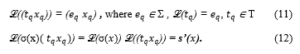
The sequence s(x)=x_0 e_1… x_(n-1) e_n x_n is a timed event sequence (T.E.S). This is the dated sequence of events, associated with the feasible dated sequence σ(x). s(x) = ℒ(σ(x)).

Definition 9: (temporal language)
Let be TLPN noted R_TL. The temporal language generated by R_TL, noted £(R_TL) is defined as all the T.E.S s(x) generated by R_TL since the initial marking m_0. £(R_TL) = {s(x) | m_0[σ(x), ℒ(σ(x)) = s(x)} where σ(x) is a dated sequence available in R_TL.

3. Failure prognosis based on TLPN

The failure prognosis is intended to predict the properties of a system that are not in compliance with the specifications. The aim is to predict the occurrence of failure events in the system before their future occurrence.

The prognosis in discrete event systems has been discussed in various research papers. Most of them have developed a prognosis approach predicting a failure event m-steps in advance, based on finite state automata [3][4][6] or Petri nets [1]-[2],[30]-[34], using stochastic and or non-stochastic ways [6][35].

Our proposed approach consists to predict a failure event n-units time in advance. The first contribution relates to a formal representation framework. The adopted modelling considers the three possible operating modes of the system, as shown in the figure 2.

• The nominal mode that contains only the set of states that represent a nominal execution of the system.
• The degraded mode groups all states in which the system operates with a tolerable degradation without influencing the behavior of the system.
• The failed mode that contains all states that represent the failed behavior of the system.

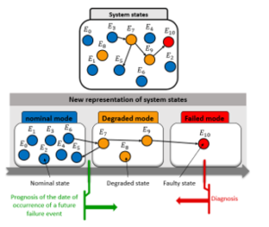
Figure 2: System states & Operating modes

Figure 2 also shows the interest of the prognosis because it aims to explain the causality. Indeed, the diagnosis cannot prevent a failure situation, whereas the prognosis offers more visibility on the future evolution of the system and makes it possible to act before a fault occurs. Our purpose consists to determine a prognosis within an operating mode managing context.

To model such behavior, we propose an extension of the Temporal Labelled Petri nets within a context of operating modes. This extension provides an ability to represent temporal constraints and labels in the modeling process. Figure 3 shows an example of operating modes of a system based on a TLPN model. Switching state is conditioned by the firing of transitions. A transition is fired if it is enabled.

The prognosis will need an observer module constrained by a place ( ) and transition ( ). This module has no influence on the behavior of the system, it only observes the occurrence time of a failure event (figure 3).

To do this, we suppose that:

• Only one transition is fired at the same time;
  • Only one mode is active at the same time;
  • The PN is safe;
  • we assume that the firing of transitions is immediate and there is no firing delay;
  • All TLPN events are observable.

 

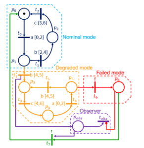
Figure 3:TLPN model with observer.

Definition 10:

The extended TLPN (ETLPN) is R_TL=<P,T,Pre,Post,m_0,Σ,L,I> where:
P= P_n ∪ P_deg∪ P_fail∪ P_obs with P_n is the set of nominal places, P_deg is the set of degraded places, P_fail is the set of failed places and P_obs is the observer place.
T= T_n ∪ T_deg∪ T_fail ∪ T_obs ∪ T_rep , the set of transitions.
If ∃p_i∈(P_n∪P_fail ) and t_j∈(T_n∪T_fail ), such that:
m(p_i)≥pre(p_i,t_j), then m(p_obs )=0 and t_obs is not enabled, otherwise, m(p_obs )=1 and t_obs is enabled.
The model of Figure 3 is an ETLPN with Σ={a,b,c,f,r}, with: f is a failure event and r is a repair event.
The transition t_6 is a failed transition such as: t_6 ∈ T_fail then,L (t_6) = f.
The transition t_7 is a repair transition such as: t_7 ∈ T_rep then,L (t_7) = r.
By firing the t_1^’ transition the system switches to a degraded mode marking thus p_obs, that is m(p_obs)=1. The p_obs place remains marked until the system switch to a failed mode.
The introduction of p_obs and t_obs doesn’t influence the behavior of the system. Their interest will be explained in the following section.
To represent sequences ending with a failure event, we use the both notions of parametric state and sequences allow to construct the reachability graph which contains only the essential states, i.e. the time associated with each timed transition enabled of a state E = (m, h) is a natural integer. However, knowing the behavior of the network in the “essential” states is sufficient to determine at any time the overall behavior of the network. (cf. [12] [22]).
The advantage of this approach is the application of linear optimization (generated by the system of inequalities in each state), which makes it possible to calculate the execution time of a sequence at the earliest and at the latest.
Clock times must be accumulated to progress from a state E of the net to a failed state E’. To do this, an observer model is introduced to the model in order to record the cumulative time between E and E’. This observer model has no impact on the behavior of the system, it just makes it possible to record the time required to progress from a non-defaulting, but not necessarily normal, to a state E’ that is considered failed.
To calculate this execution time, we propose an extension (definition 11) of definition 5. But before discussing the proposed approach, we formulate the following assumptions:
The system model is known all events are observable. The case of prognosis under partial observation is not considered here.
The prognosis begins when the model switches from nominal mode to degraded one.
Remark: the remains the same, if the prognosis is started from any nominal state of the system.
The following framework (figure 4) describes the steps of the proposed prognosis approach. The first step, called the behavioral model, is required to describe the possible operating modes of the system (figure 3). The prognoser is an oriented state graph (figure 8), built from the system model, its role is to detect all possible traces ending with a failure event; Once the system switches from nominal to degraded mode, the prognoser must identify all the sequences of the model namely those that lead to a failure event. Such an event cannot be predicted overall in the sequences. The prognosability property is introduced to determine the sequences of failure event that can be predicted. From an inequality system, the execution time of each sequence is calculated; It called “Time signatures of execution traces”. The minimal time signature will then represent the earliest date before a failure event occurs.

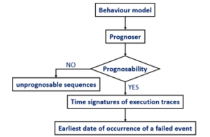
Figure 4: Framework

In fact, the prognosis is not possible, when two traces σ_1 and σ_2 have the same time constraints and the same sequencing of events. For example, in figure 6, σ_1= t_1.1…t_n, σ_2= t_2.1…t_m and
s_1 (x)=x_1.0 e_i x_1.1…x_(1.n-1) e_n x_(1.n),
s_2 (x)=x_2.0 e_j x_2.1…x_(2.m-1) fx_(2.m)(with ? a failure event) are their respective parametric event sequences.

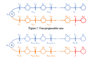
Figure 6: Prognosable case

Deciding on the future execution of σ_1 or σ_2 from a state ? is conditioned by:
Pre(•, t_i )≤m_0∨Pre(•, t_j )≤m_0 ∧t_i≠t_j i.e. t_i and t_j are enabled from ?.
e_i∈∑_o∨e_j∈∑_o∧e_i≠e_j, otherwise if e_i=e_j it is required that I_(x_1.0 )∩I_(x_2.0 )=0 (I_(x_1.0 ) execution interval of x_1.0)
In other case, we cannot prognosticate the failure event f.

If we consider in figure 5 that e_i=e_j, the failure event f cannot by prognosable. But if e_i=e_j and the intervals of the dated sequences are different then the failure event f is prognosable (figure 6).

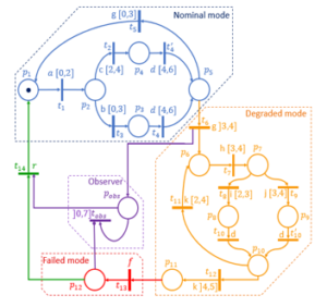
Figure 7: Model 2

The resolution of the inequation system will be the last step, which calculates the time signature of execution for all the prognosable sequences. The minimum execution generated from this step represents the earliest occurrence time of a failure event.

In the example shown in figure 7, the prognosis starts from the firing transition  because degraded mode will start at this place.

Indeed, if the event g occurs at earliest after 3 units time, the model switch to the degraded mode. From this state the observer place ( ) will be activated, and its corresponding transition  becomes enabled until the event f (failure event) will occurred. Thus, the interval times associated with the transitions enabled from place , will be combined in the form of associated system of inequalities to  while the occurrence of the failure event ? of the transition  does not occur. When the event r is generated (meaning that the system is repaired), the observer place will be initialized to allow a next operating cycle.

The place is called the candidate place for the prognosis. Once this place is marked, the occurrence of the failure event can be predicted.

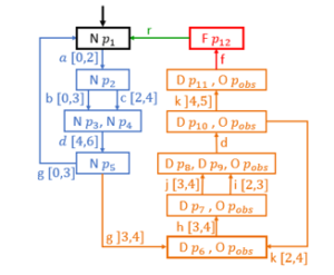
Figure 8: Prognoser model.

Figure 8 link to model 2 presents the prognoser model where a state is composed by the marked states of the model and their corresponding mode the nominal states are represented by N, degraded by D and failed states by F, except for Pobs place that will be associated to Observer module noted O. The prognosis of the event occurrence date is possible from any state of the prognoser. {N } for example, represent a marking of the system and its corresponding operating mode, i.e.  indicates that the place  is marked and N indicates that the system is in nominal mode. The occurrence of event g in interval ]3,4] leads the prognoser model to {D ,O } where  and  are the marked places and D means that the system is in degraded mode and is marked. When the prognoser switches to a state with  place marked, the prognosis process is then activated. The prognosis process is achieved by the identification of all sequences ending with an F state. According to the prognoser’s model and from {D ,O } the event sequences ending in a failure event are:  and .To simplify, we don’t take into consideration  and  cycles.

Then, the execution time of each sequence is calculated (time signature) by applying algorithm 2. The aim is to find all the minimum solution values of the system of inequalities. These values will constitute the minimum time after which the occurrence of the failure event is certain.

Definition 11, which is an extension of definition 5, allows, from a TLPN, to recursively determine the parametric state and parametric sequence leading to a failure state, and thus generating the system of inequalities composed of the constraints obtained from the intervals associated with each enabled transition from a candidate place. But before presenting definition 11, let’s first reconsider a set of enabled transitions from a  marking.

Let m be a marking of a PN. We define V_m the set of enabled transition from m as follows: V_m={t_i ” T” │” ” m”  Pre(” •”,” t_i “)” },
Definition 11: (parametric state and sequence of an TLPN)
Let R_TL=<P,T,Pre,Post,m_0,Σ,L,I> a TLPN, m a p_marking and h a t_marking containing the time associated with each transition enabled from m. σ:=t_1…t_n is a firing transition sequence in R_TL and σ(x):=x_0 t_1… x_(n-1) t_n x_n its feasible dated sequence. V_(m_σ ) is the set of transitions enabled from the m_σ marking (final marking) obtained by the firing of the transition sequence σ.
Then, the parametric sequence (σ(x),B_σ) of σ and the parametric state (E_σ,B_σ) in R_TL are determined by the algorithm 1.

Algorithm 1 Prognosis algorithm
Begin
* if σ = ε, i.e. σ(x)= x_0 and s(x)=x_0
Then E_σ=(m_σ,h_σ) and B_σ are given by:
m_σ≔m_0,
V_(m_σ )=V_(m_0 )={t_i ┤| m_0 ” “” Pre(“•”,” t_i “)}”
h_σ (t)=h_0 (t)={█(█(x_0 &if Pre(•,t)≤m_0@$ &Otherwise))┤
B_σ≔ {0  h_σ (t)  max(t) | t ∈ T ∧ Pre(•, t) ≤ m_σ}
Else
repeat
We assume that E_σ and B_σ are already defined for the transition sequence σ:=t_1…t_n.
then σ(x):=x_0 t_1… x_(n-1) t_n x_n. its corresponding T.E.S is s(x)=x_0 e_1… x_(n-1) e_n x_n for σ:=t_1…t_n t_(n+1) = t_(n+1), and
ℒ(σ) = ℒ().ℒ(t_(n+1)) = s(). ℒ(t_(n+1))
1. m_σ≔m_γ + Δt_(n+1), with Δt_(n+1) := Post(•,t_(n+1) ) – Pre(•, t_(n+1) )
2. V_(m_σ )= {t”| ” m_σ ” “” Pre(“•”,” t”)}”
3. h_σ (t)={█($ “if” Pre(•,t)≰m_σ @h_γ (t)+x_(n+1) “if” Pre(•,t)≤m_σ∧Pre(•,t)≤m_γ@ ∧Pre(“t” _”n+1″ )”∩Pre(t) = ∅  t ≠ ” “t” _”n+1″ @x_(n+1) ” Otherwise” )┤
4. B_σ := B_γ ∪ {min(t_(n+1))  h_γ(t_(n+1))} ∪ { 0 ≤ h_σ(t) ≤ max(t) | t ∈ T ∧ Pre(•, t) ≤ m_σ }
until (ℒ(t_(n+1)) = ef)
End
Let the TLPN of Figure 7 and apply definition 11
At the start  : =  , σ(x)= x_0;
E_σ=(m_σ,h_σ )=(m_0,h_0 ) ;
m_0=(p_1 )^T, means that only p_1 is marked with 1 token and 0 token in the rest of the other places;
V_(m_0 )={t_1 };
ℒ(t_1) = a;
h_0 (t)=〖(x_0,$,$,$,$,$,$,$,$,$,$,$,$,$,$,$,$)〗^T;
B_0={0≤x_0≤2}.
σ= t_1 ;
m_1=(p_2 ),
V_(m_1 )={t_2 〖,t〗_3}, means that only t_2 and t_3 are enabled from the marking m_1;
ℒ(t_2) = b, ℒ(t_3) = c;
h_1 (t)=〖(〖$,x〗_1,x_1,$,$,$,$,$,$,$,$,$,$,$,$,$,$)〗^T;
B_1 ={█(0≤x_0≤2@0≤x_1≤3)}
σ= t_1 t_3 ;
m_2=(p_3 )^T; V_(m_2 )={t_4 } ;
ℒ(t_4) = d;
h_2 (t)=〖($,$,$,x_2,$,$,$,$,$,$,$,$,$,$,$,$,$)〗^T;
B_2={█(0≤x_0≤2@0≤x_1≤3@0≤x_2≤6)}
σ= t_1 t_3 〖 t〗_4 ;

m_3=(p_5 )^T; V_(m_3 )={t_5 〖,t〗_6 } ;

ℒ(t_5) = ℒ(t_6) = g;
h_3 (t)=〖($,$,$,$,x_3,x_3,$,$,$,$,$,$,$,$)〗^T;
B_3={█(0≤x_0≤2@0≤x_1≤3@4≤x_2≤6@0≤x_3≤3)}
σ= t_1 t_3 〖 t〗_4 〖 t〗_6;
m_4=(p_6 p_obs )^T,V_(m_4 )={t_7,t_obs } ;
ℒ(t_7) = h;
h_4 (t)=〖($,$,$,$,$,$,x_4,$,$,$,$,$,$,$,$,$,x_4)〗^T;
B_4 ={█(0≤x_0≤2@0≤x_1≤3@4≤x_2≤6@3≤x_3≤3@0≤x_4≤4)}

σ= t_1 t_3 〖 t〗_4 t_6 t_7;

m_5=(p_7 p_obs )^T,V_(m_5 )={t_8,t_9 〖,t〗_obs } ;

ℒ(t_8) = i, ℒ(t_9) = j;

h_5 (t)=〖($,$,$,$,$,$,$,x_5,x_5,$,$,$,$,$,$,$,x_4+x_5)〗^T;
B_5={█(0≤x_0≤2@0≤x_1≤3@4≤x_2≤6@3≤x_3≤3@3≤x_4≤4@0≤x_5≤3@x_4+x_5≤7)}
σ= t_1 t_3 〖 t〗_4 t_6 t_7 t_8;
m_6=(p_8 p_obs )^T,V_(m_6 )={t_10 〖,t〗_obs } ;
ℒ(t_10) = d;
h_6 (t)=〖($,$,$,$,$,$,$,$,$,x_6,$,$,$,$,$,$,x_4+x_5+x_6)〗^T;
B_6={█(0≤x_0≤2@0≤x_1≤3@4≤x_2≤6@3≤x_3≤3@3≤x_4≤4@2≤x_5≤3@0≤x_6≤0@x_4+x_5≤7@x_4+x_5+x_6≤7)}
σ= t_1 t_3 〖 t〗_4 t_6 t_7 t_8 t_10;
m_7=(p_8 p_obs )^T,V_(m_7 )={t_11,t_12,t_obs } ;
ℒ(t_11) = ℒ(t_12) = k;
h_7 (t)=〖($,$,$,$,$,$,$,$,$,$,x_7,x_7,$,$,$,$,x_4+x_5+x_6+ x_7)〗^T;
B_7={█(0≤x_0≤2@0≤x_1≤3@4≤x_2≤6@3≤x_3≤3@3≤x_4≤4@2≤x_5≤3@0≤x_6≤0@0≤x_7≤4 @x_4+x_5≤7@x_4+x_5+x_6≤7@x_4+x_5+x_6+x_7≤7)}
σ= t_1 t_3 〖 t〗_4 t_6 t_7 t_8 t_10 t_12 ;
m_8=(p_11 p_obs )^T,V_(m_8 )={t_13,t_obs } ;
ℒ(t_13) = f;
h_8 (t)=〖($,$,$,$,$,$,$,$,$,$,$,$,x_8,$,$,$,x_4+x_5+x_6+〖 x〗_7+x_8)〗^T;
B_8={█(0≤x_0≤2@0≤x_1≤3@4≤x_2≤6@3≤x_3≤3@3≤x_4≤4@2≤x_5≤3@0≤x_6≤0@4≤x_7≤4@0≤x_8≤0@x_4+x_5≤7@x_4+x_5+x_6≤7@x_4+x_5+x_6+x_7≤7@x_4+x_5+x_6+x_7+x_8≤7)}
We obtain the system of inequalities B_8. It is necessary to find all the minimum solution values of this system of inequalities. See the solution in table 1:

Table 1:The Inequation System Solution.

0	0	4	3	3	2	0	4	0	12

To do this, we follow the next steps:

• Give real values that are solutions of the system of inequalities .
• Calculate the minimum integer values that always check the system of inequalities without changing the behavior of the system.

We considered the smallest possible values for each .

Thus, from the candidate place P₆, we will reach the failure state (place P₁₂) after at least 12-time units. We assume that only one cycle is executed in degraded mode. We can, of course predict the failure state from any nominal or degraded state.

4. Conclusion

In this paper, we have presented two contributions to determine the prognosis of a failure event in discrete event systems. The first one is about the exploitation of the technique of state and events sequence parametrization on a model of temporal labelled Petri nets. The interest is to reduce the state space of the model for an analysis of both the order and the date of occurrence of events. The second contribution is the proposal of an algorithm based on a system of inequations, to determine the occurrence date of a future failure event. The proposed algorithm makes it possible to determine, from a place belonging to all the candidate places, the minimum date necessary to reach a critical place from which the occurrence of the failure event is certain.

Work in progress considers the system under partial observation, which makes it possible to address the problem of the system’s prognosability.

Works presented in this paper supposed that the used PN is safe, but in practice, the system is composed of several components, it would then be more interesting to consider a multi-token model and assign a type of clock according to the nature of the token and then to predict the failure status for each component in the same model.

It would also be very important to predict the failure event of a system while considering the aging state of the system.

1. R. Ammour, et al. “Fault prognosis of timed stochastic discrete event systems with bounded estimation error” Automatica 82 (2017): 35-41.
2. R. Ammour, et al. “Faults prognosis using partially observed stochastic Petri-nets: an incremental approach” Discrete Event Dynamic Systems 28.2 (2018): 247-267.
3. J. Chen, R. Kumar, “Failure prognosability of stochastic discrete event systems” 2014 American Control Conference. IEEE, (2014).
4. S. Takai, “Robust failure prognosis of partially observed discrete event systems” 2012 American Control Conference (ACC). IEEE, (2012).
5. P. Merlin, “A study of the recoverability of communication protocols” PhD Theses, Irvine (1974).
6. A. Khoumsi, “Alternative Inference-Based Decentralized Prognosis of Discrete Event Systems” In 2019 6th International Conference on Control, Decision and Information Technologies (CoDIT) (pp. 250-255). IEEE (2019, April).
7. Z. Ma, et al. “Marking Estimation in Labelled Petri nets by the Representative Marking Graph” IFAC-PapersOnLine 50.1 (2017): 11175-11181.
8. A. K. A. Toguyeni, “Surveillance et diagnostic en ligne dans les ateliers flexibles de l’industrie manufacturière” (Doctoral dissertation, Lille 1) (1992).
9. Y. Pencolé, “Diagnostic: étude d’un raisonnement complexe et multi-dimensionnel” (Doctoral dissertation 2018).
10. R. Saddem, “Diagnosticabilité modulaire appliquée au Diagnostic en ligne des Systèmes Embarqués Logiques” (Doctoral dissertation 2012).
11. L. Popova-Zeugmann, “Time and Petri Nets” Springer, Berlin, Heidelberg, (2013). 31-137.
12. Popova-Zeugmann, “Time and Petri Nets” DOI 10.1007/978-3-642-41115-1_3, © Springer-Verlag Berlin Heidelberg (2013).
13. L. Popova-Zeugmann, “On parametrical sequences in time Petri nets” Proceedings of the CS&P. Vol. 97. (1997).
14. B. Berthomieu, et al. “Problèmes d’accessibilité et espaces d’états abstraits des réseaux de Petri temporels à chronomètres.” Journal européen des systèmes automatisés 39.1/3 (2005): 223.
15. B. Berthomieu, M. Diaz, “Modeling and verification of time dependent systems using time Petri nets” IEEE transactions on software engineering 3 (1991): 259-273.
16. B. Berthomieu, M. Menasche, “An enumerative approach for analyzing time Petri nets” Proceedings IFIP. (1983).
17. B. Berthomieu, “La méthode des classes d’états pour l’analyse des réseaux temporels” 3e congrès Modélisation des Systèmes Réactifs (MSR’2001). (2001).
18. B. Berthomieu, “Réseaux de Petri temporels” ETR septembre (2003): 123-153.
19. B. Berthomieu, F. Vernadat, S. D. Zilio, “TINA: Time Petri Net Analyzer” (2015).
20. L. Popova-Zeugmann, “On time Petri nets” Journal Information Processing and Cybernetics, EIK 27.4 (1991): 227-244.
21. L. Popova-Zeugmann, “On liveness and boundedness in time Petri nets” Proceedings of the Workshop on Concurrency, Specification and Programming (CS&P’95). (1995).
22. L. Popova-Zeugmann, “Essential states in time Petri nets” Humboldt-Univ. zu Berlin, (1998).
23. P.J Ramadge, W.M. Wonham, “the controle of discrete-event systems” Proc. IEEE, vol. 77, no 1, pp 81-98, (1989).
24. B. Bérard et al. “Comparison of different semantics for time Petri nets” International Symposium on Automated Technology for Verification and Analysis. Springer, Berlin, Heidelberg, (2005).
25. B. Berard et al. “The expressive power of time Petri nets” Theoretical Computer Science 474 (2013): 1-20.
26. D. Lefebvre, “Fault diagnosis and prognosis with partially observed Petri nets” IEEE Transactions on Systems, Man, and Cybernetics: Systems 44.10 (2014): 1413-1424.
27. F. Basile, P. Chiacchio, J. Coppola, “Identification of labeled time Petri nets” 2016 13th International Workshop on Discrete Event Systems (WODES). IEEE, (2016).
28. F. Basile, P. Chiacchio, J. Coppola, “Identification of time Petri net models” IEEE Transactions on Systems, Man, and Cybernetics: Systems 47.9 (2016): 2586-2600.
29. V. D. Aalst, W. M. P. “Timed Coloured Petri Nets and their Application to Logigcs” Diss. PhD thesis, Tech. Univ. Eindhoven, (1992).
30. D. Lefebvre, “Fault diagnosis and prognosis with partially observed stochastic Petri nets.” Proceedings of the Institution of Mechanical Engineers, Part O: Journal of Risk and Reliability 228.4 (2014): 382-396.
31. D. Lefebvre, “Fault diagnosis and prognosis with partially observed stochastic Petri nets.” Proceedings of the Institution of Mechanical Engineers, Part O: Journal of Risk and Reliability 228.4 (2014): 382-396.
32. M. Ghazel, “Surveillance des systèmes à évènements discrets à l’aide des réseaux de Petri Temporels” Diss. Ecole Centrale de Lille, (2005).
33. R. Ammour, et al. “Faults prognosis using partially observed stochastic Petri nets” 2016 13th International Workshop on Discrete Event Systems (WODES). IEEE, (2016).
34. F. Basile, P. Chiacchio, G. De Tommasi. “Fault diagnosis and prognosis in Petri Nets by using a single generalized marking estimation” IFAC Proceedings Volumes 42.8 (2009): 1396-1401.
35. D. Lefebvre, “Fault diagnosis and prognosis with partially observed Petri nets” IEEE Transactions on Systems, Man, and Cybernetics: Systems 44.10 (2014): 1413-1424.

(Click Here)

(Click Here)