1. Introduction

The purpose of this paper is to demonstrate the application of Causal Modeling in the domain of Cybersecurity. We engage in the scientific inquiry into the underlying causes of data breaches. Using methods of causal analysis that link concepts to observations, and a rationale connecting concepts to practice. The notion of causality, as used in Computer Science, provides principles that guide the problem specification, elaboration of the procedures, and interpretation of datasets. We employ causal modeling for the purpose of providing a computable measurement of a certain group of data breaches.

We tackle a variety of data breach problems that affect our industries and have an impact on the overall economy.  In our work, we demonstrate how the usage of Causal Modeling can help us locate such data breach problems.  Statistical analysis is enough for identifying associative relationships. While this is useful for general analysis, Causal Modeling provides a different structure with interventions included in it.  Interventions tell us what would have happened if events other than the ones we are currently observing had happened.  Such interventions allow us to avoid unnecessary steps and come directly to the point. It can also provide justification as to why and how the desired step or conclusion is arrived and provide defense for potential future cases. In order to intervene, we needed to estimate the effect of changing an input from its current value, for which no data exists. Such questions, involving estimating a counterfactual, are common in decision-making scenarios.

      Statistical Prediction is the estimation of an outcome based on the observed association between a set of independent variables and a set of dependent variables. Its main application is forecasting.

Causality is the identification of the mechanisms and processes through which a certain outcome is produced. It can be used in predicting future events that are similarly connected via mechanisms and processes. Causal relations are not features that can be directly read off from the data, but have to be inferred. The field of causal discovery is concerned with this inference and the assumptions that support it.

Our research focuses on two aspects of Causal Modeling: Causal Discovery and Causal Inference. Causal Discovery algorithms try to derive causal relations from observational data. Given a set of data, a causal discovery algorithm returns a set of statements regarding the causal interactions between the measured variables.

Causal Inference is the process of drawing a conclusion about a causal connection based on the conditions of the occurrence of an effect. The main difference between causal inference and statistical inference of association is that the former analyzes the response of the effect variable when the cause is changed. The process shows causal direction, which is rarely found by statistical correlation alone. For example, a question that  causal reasoning can answer is: Is there a causal link between the distribution across values of a certain variable X and values of another variable Y?

Causal inference process solves causal problems systematically, by methods such as counterfactual analysis, graphical models, and the association between counterfactual and graphical methods.

Causal modeling resolves questions about possible causes by providing explanation of phenomena as the result of previous events. One can generate a plausible explanation for gaps within cybersecurity infrastructure.  The usage of Causal Modeling can help us locate a set of data breach problems and help provide a solution for such problems.

The objective of this research is to evaluate the risks of data breach  of cybersecurity incidents with the overall aim to identify patterns of importance amongst the dataset, accomplished by noting causes and effects in the modeling process. This is achieved by studying the characteristics of the VERIS Community Database (VCDB) of cybersecurity incidents. VCDB is a widely used open-source dataset containing a breadth of information regarding data breaches.

2. Background

We offer a scientific method based on the notion of causation. Following are the motivations behind the use of Causal Modeling for Cybersecurity:

One can draw from past experiences, and try to build a probability distribution [1]. Standard probability theory has been productive in these problems and similar ones, when the past experiences are readily available for analysis. But there are instances where it fails to provide adequate concepts and mathematical methods, particularly when the past experiences are either not available, or are not relevant.

A context like breach of data can interact with the phenomena of interest in ways that standard probability theory does not productively capture; that is, in ways that standard probability theory does not provide insights and methods for useful modeling and fails to capture key concepts.  Some of these key concepts are the necessary and sufficient conditions that produce the essential model of the cause-effect relationships involved.

A necessary condition is one that is required if a certain effect is to follow. A sufficient condition, on the other hand, is enough for certain effects to follow.

Some of the usage of the necessary and sufficient conditions are as follows: we have to look for causes that are common in the cases where the effect also occurs. Thus, some event is not a necessary condition if it happens without the effect occurring [2,3].

We can explore causal modeling on observational data.  In general, to determine whether or not an uncertain variable x_k (the supposed effect) is responsive or unresponsive to decision d we have to answer the query “Would the outcome of x_k have been the same had we chosen a different alternative for d?” Questions of this form are counterfactual queries [4,5].

   We define the Counterfactual World as follows.  there are some uncertain variables, X (of which x_k is an instance), such as data leakage (including some uncertainty as to why, and are we sure about the leakage?)  in the scenario; there is also the set of  potential causes C [6].  Possible candidates for the causes in C are:

• malware in the system
• hacking
• human error

Let U be the total set of possible effects pertaining to some scenario S.  These are possibilities that should be determined correctly. There are variables  X ⊆ U, which are uncertain variables.  We also have a set of decisions D (for example, the decision that the data leakage  is, indeed, there, and that it is there because of the bugs). Given these notions, the concept of counterfactual world can be defined.  A counterfactual world of X and D is any instance of such world retained by X ∪ D, after the decision maker selects a particular instance of  D [7].

Definitions of unresponsiveness and responsiveness are to be understood next. Suppose that we have some uncertain variables, which form a set X. Also, suppose that we have a set of decisions D. There can be counterfactual worlds  D that can form union with the set X.  D is the set of scenarios where there is  a list of counterfactual decisions (and the outcomes associated with the decisions), which may never take place in the real world as we encounter it. X is unresponsive to D, denoted as X  ↚ D, if X assumes the same instance in all counterfactual worlds of X ∪ D [8]. That is, instances of  X do not affect  the status of X ∪ D. In the case of Cybersecurity, an example of a counterfactual world can be one in which no cybersecurity compromise is ever reported. These counterfactual variables are not observed, and, most probably, will never be observed. Examples of X can be concerns about Cybersecurity. These two can form a union,  but X is unresponsive to D,  since the instances of such concern do not affect the union. In contrast, one can think of a set X as being responsive to a set D. In this case, let the set X be the same as before, namely, the set of concerns about Cybersecurity, for example, concerns about data leakage as an element of X. The counterfactual world D can be one where Cybersecurity compromise is supposed to be reported to computer users, but ignored.

If concerns about the data leakage problem is an example of X, then it can assume different instances in different counterfactual worlds of X U D.

For example, “If one had this concern about data leakage, then one may or may not have ignored the Cybersecurity compromise report”.

This shows that some instances of X can belong to some counterfactual world of X U D. Therefore, X is responsive to D.

X refers to the collections of events (indicating, for example, different states of data leakage) some of which occur after decision(s) D have been made. Given decisions D, the variables in the set C are causes of x with respect to D if all the following three conditions are met:

• Condition 1: x is not a member of C.
• Condition 2: x is responsive to D.
• Condition 3: C’ is a minimal set of variables such that x is unresponsive to D in worlds limited by C’ (that is, x ← D, and C’ is a minimal set such that x ↚ c’ D).

The third condition is saying that C has a definite influence on x being responsive to D. The influence is that the relevant cause (or causes) must be included in whichever set of variables that also necessarily differ (being responsive) in accord with x being responsive to D.  So, the set C’ that limits the relation of x with D (regarding responsiveness) is a minimal set.

The following are the brief explanations with regard to the system discussed here.

• Condition 1 affirms that the effect (X) is not a member of the set of causes.
• Condition 2 affirms that for x (data leakage) to be caused with respect to decision D (data leakage must have been caused by the bugs in the system), it must be responsive to that decision.
• Condition 3 states the following: suppose that one can find a set of variables Y such that X, data leakage, can be different in different counterfactual worlds only when Y is different.  In that case, Y must contain a set of

Our approach in this paper is showing the effects of intervention. Causal modeling  helps us ask the right questions about causation and helps us devise a way to emulate it by means that are not intrusive. Our emulation of interventions  are based on observational studies and using data to find causal relation between them.

Causal relations are not features that can be directly read off from the data, but have to be inferred. The field of causal discovery is concerned with the inference and the assumptions that support it. Instrumental variable method ensures that we obtain the close-to-correct causal effect, even if there are unobserved conditions.  Combining propensity-based and regression-based methods provides us with a causal estimate that is accurate whenever the model is correctly specified.

The potential outcomes framework can be detailed as follows: counterfactual variables such as “knowledge and action of a person P had  he received the information that the cybersecurity of his computer system has been compromised ”and “knowledge and action of a person P had he not received the information that the cybersecurity of his computer system has been compromised” are as appropriate as traditional variables such as “knowledge and action of a person P” – though one of these counterfactual variables is not observed, and most probably, will never be observed, in the case of this person P .

2.1.   Common Cause, Confounding, Control, and Instrumental Variables.

Common causes explain the fact that there are concepts related to causation that are more important than correlation.

Suppose that a person has received a “Compromised Host” notice from some authorities, and also his computer-savvy friend (who may or may not know about the notice) has checked this person’s computer and is confident that attackers have gained unauthorized access to this person’s computer. Therefore, this person is worried about cybersecurity, and would like to take steps.

What are the causes of receiving such as notice? What are the causes of this computer-savvy friend being confident that attackers have gained unauthorized access to this person’s computer? If there is some disaster, it could cause the “Compromised Host” notice  to go out. It could also cause one’s computer-savvy friend being confident that attackers have gained unauthorized access to this person’s computer.

If a disaster happens, both of these are likely. This means in a data set one can find a correlation between the two.

We know there is no causal effect of receiving a “Compromised Host” notice  on one’s computer-savvy friend (who may or may not know about the notice) being confident that attackers have gained unauthorized access to this person’s computer, or vice versa. This is the essence of “correlation does not imply causation”.

When there is a common cause between two variables, then the variables will be correlated. This is part of the reasoning behind the phrase, “There is no correlation without causation”.

Suppose that we are dealing with two concepts, named A and B. If neither A nor B has been definitely known to cause the other, and the two are correlated, there must be some common cause of the two. It may not be a direct cause of each of them, but it is there somewhere. This implies that we need to control for common causes if we are trying to estimate a causal effect of A on B.

Common cause variation is fluctuation caused by unknown factors resulting in a steady but random distribution of output around the average of the data.

Suppose that we take the average of the data, and do a steady but random distribution of output around the average. There will be unknown factors that will result in that distribution. This will cause a source of variation called common cause variability. This is a measure of  the potential of the process – which includes how well the process can perform, if and when special cause variation is removed.  Common cause variation is also called random variation, or non-controllable variation.

If we do not include hidden common causes in our model, we will estimate causal effects incorrectly. This is similar to the notion of confounders (in this particular case, some cybersecurity disaster has happened).

Confounding variables are to be understood in terms of data generating model. Pearl defines the concept of confounding as follows: Let X denote some independent variable (for example, the “Compromised system “notice), and Y some dependent variable (the person is worried and wants to take action). We might want to estimate what effect X has on Y, without regard to other potential factors; for example, if the person is, at the same time, not feeling well. We say that X and Y are confounded by some other variable Z whenever Z is a cause of both X and Y. In our case, Z is that some cybersecurity disaster has happened.

One can state that X and Y are not confounded whenever the observationally witnessed association between them is the same as the association that would be measured in a controlled experiment, with x randomized.

An equality here can be stated as P(y | do(x)) = P(y | x); this can be verified from the data generating model provided that we have all the equations and probabilities associated with the model. This is done by simulating an intervention do (X = x) and checking whether the resulting probability of Y equals the conditional probability P (y | x).

Control is a concept related to confounders. Suppose that we are attempting to assess the effectiveness of the notice being given, from population data. The data shows that prior knowledge about such incidents (Z) influences the state of mind .e.g. worry and wanting to take action (Y). In this scenario, Z confounds the relation between X (his computer-savvy friend takes the action of  telling him) and Y since Z is a cause of both X and Y.

We hope to obtain an unbiased estimate P(y | do(x)) = P(y | x). In cases where only observational data are available, an unbiased estimate can only be obtained by “adjusting” for all confounding factors, which means conditioning on their various values and averaging the result.

This gives an unbiased estimate for the causal effect of X on Y. The same adjustment formula works when there are multiple confounders except, in this case, the choice of a set Z of variables that would guarantee unbiased estimates must be done with care. One can view cause-effect relationships via directed acyclic graphs; one should also link causal parameters and observed data, such as information about the subjects studied, as well estimation of the resulting parameters.

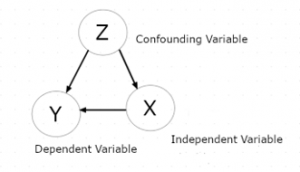
Figure 1. Example of a Causal Model

3. Overview

Since experimentation is not feasible for simulating real world data breaches, the analysis relies solely on observational data. In this regard, Judea Pearl’s theory of Counterfactual World theory is extended with the use of propensity scores to calculate causal inference. The main issue to tackle regarding the use of observational data is the bias within the data caused by confounding variables, both known and unfounded. These include the previously mentioned common causes, instrumental variable, and any other covariates.

We thus present the use of causal modeling as a tool for gaining insight into how data breaches occur, and the degree to which certain associations behind these breaches can be seen as causal. We present a subset of open-sourced data offered by Verizon Communication. We then apply principles of Pearlian Causal inference through the software library DoWhy in order to understand the causal effects of our interventions.

3.1.  Methodology

We concluded that DoWhy, a Microsoft open source Causal Modeling framework, was most appropriate for this current project, for its ease of use and abundant resources. It also provided an intuitive method to implement the Model -> Identify -> Estimate -> Refute structure of the analysis. All of these were readily provided by DoWhy and were thus implemented with DoWhy’s built-in functions. Due to the limitation on data availability regarding data breaches, we believe these provided enough for an exploratory analysis on the subject [9,10].

DoWhy also provides a principled way of modeling a given problem as a causal graph so that all assumptions are unequivocal and explicit. It provides an integrated interface for causal inference methods, combining the two major frameworks of graphical models and potential outcomes. It also automatically tests for the validity of assumptions if possible and assesses the robustness of the estimate to violations.

It is important to note that DoWhy builds on two of the most powerful frameworks for causal inference: graphical models and potential outcomes. It uses graph-based criteria and do-calculus for modeling assumptions and identifying a non-parametric causal effect. For estimation, it switches to methods based primarily on potential outcomes.

In the following paragraphs we will describe the techniques to use for our analysis: Propensity Score Matching, Propensity Score Stratification, and Linear Regression Estimator. These techniques can all be founded within the DoWhy framework.

Linear Regression Estimator provides a baseline analysis assuming an evenly distributed dataset. It provides a foundation to compare results with the other methods. As linear regression only describes a correlation between the treatment and outcome, Propensity Score Matching and Propensity Score Stratification both use linear regression while adding additional processes in order to account for confounding variables and properly compartmentalize each data entry to find a causal relationship between the treatment and outcome.

Propensity Score Stratification takes the propensity scores of each entry and classifies them into equal sub-groups. These subgroups are classified by the similarity of the covariates. The aim is to have each sub-group represent a distribution that accurately represents a non-biased dataset to the best of its ability.

Propensity Score Matching instead takes the propensity scores of each entry and finds the entries with the highest propensity scores within the treatment group and finds the entries within the control group with covariates that most closely match each treatment group entry. This attempts to establish parity between the covariates of the treatment group and the control group.

Both Matching and Stratification work to remove bias from high-dimensional datasets. They do so by balancing out the treated and control groups with processes that emulate a random distribution in an experiment. This is done by evaluating the propensity score of each group. The propensity score represents the probability of the treatment on each sample in the treatment group and is calculated by mapping the outcomes to a linear regression line. The difference in the methods in how they use the propensity score to balance out the treatment and control group.

In addition, refuters are necessary in the causal analysis process in order to verify the robustness of the results. The following methods all check the effects of confounding variables and compare them with the treatment to concretely establish a causal relationship. Generally, the refuters all involve rerunning the same causal analysis methods with the following changes to the dataset:

• Placebo Refuter: Replaces the treatment variable with a placebo variable with random values
• Data Subset Refuter: Runs the program over a randomly chosen subset of the original data
• Common Cause Refuter: Generates a random confounding variable

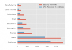
Figure 2: Number of Data Breaches by Industry

3.2.   Data Acquisition

We note that high-quality information on real-world cybersecurity incidents through academic or otherwise publicly accessible channels is likely to be unrepresentative of the nature in which breaches occur on a broader scale. As a result, we focus on analyzing healthcare privacy breach data, which generally enjoys stringent reporting standards. Our reasoning is as follows.

For the private sector, disclosure of breaches can negatively impact short term company value as well as consumer trust. A report by IBM’s Ponemon Institute in 2019 estimates the global average impact of having a data breach to an organization to be 3.9 million US dollars, representing a rise of 12% over the course of five years. For organizations with fewer than 500 employees, this cost averages to 2.5 million dollars [11]. Voluntary disclosure of data breaches may be unpalatable in light of this [12].

In contrast, government and healthcare institutions are generally under greater legal pressure to disclose similar incidents. For instance, the Department of Human and Health Care Services (HHS) in the United States mandates that information regarding data breaches involving over 500 individuals be disclosed to the media within 60 days of discovery. Structured collection of such breaches is made publicly available through the HHS website [13].

Initial exploration was performed on the VERIS Community Database (VCDB). The VCDB is an open dataset covering a broad spectrum of security incidents occurring throughout both public and private sectors. Data available through this channel represents a small portion of data contained in a more comprehensive report presented in Verizon’s annual Data Breach Investigation Report. The VCDB is attractive as there are few publicly available repositories containing annotated security breach information [14].

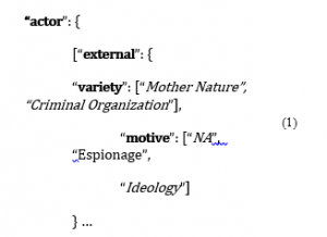
The VCDB follows the Vocabulary for Event Recording and Incident Sharing (VERIS) framework. Generally, information surrounding security incidents is divided into four categories: Actor, Attribute, Asset, and Action. Actor pertains to the entity or entities responsible for the data breach. Asset characterizes the type of information lost, as well as how accessible said information was. Attribute refers to the degree which the asset in question was affected, as well as the severity of the incident, the medium of transmission, and if said data was exposed to the public. Finally, Action describes how the security breach was carried out; such as if the breach was a result of malware, or simply negligence. Additional data on affected industry and incident timeline are included as well.

To accommodate the wide variety in reporting standards, VERIS uses a fine-grained approach for characterizing security incidents, using a nested key-value store to accommodate some 173 attributes.

We will take the “actor” category as an example. For any given incident, the individual or individuals responsible could be categorized as either external, internal (affiliated with the organization), a partner (associate, but not directly affiliated), or simply unknown or not available. Within each type of actor lies a different subcategory. For instance, the “external actor” label can represent a criminal organization, foreign government, former employee, or a combination thereof. As a result, many of the keys contain lists as values, as represented in (1).

3.3.  Why Healthcare?

While the VCDB contains many features describing the companies that were victims of data breach, little information seems to be provided regarding the situation preceding and during the data breach. Therefore, to maintain a degree of uniformity of each company, narrowing down to one industry like healthcare would mitigate discrepancies within the dataset.

Furthermore, the VCDB utilizes a JSON-formatted, hierarchical data structure presented as a list of key-value pairs.  While each record adheres to the same general schema, sparsity arises as a result of how much data is disclosed by each entity, or simply what information is relevant to which sector. Referring back to US Healthcare data breach disclosure law, we can expect a baseline of data to be provided, such as the number of individuals affected, the type of breach, and the vector of attack.

The next logical step was to transform the data from a hierarchical format into a two-dimensional, tabular structure. A strong motivation for this was to make the data both more comprehensible and consistent.

Transforming the database for VCDB was straightforward thanks to the open-source library Verispy. Verispy converts the deeply nested structure of the original VCDB dataset into a two-dimensional grid-like format. by performing “one-hot encoding” on each of the categorical variables.

This leads to a relatively consistent dataset with the caveat of vastly increasing the (perceived) dimensionality. The final table consists of 2,347 columns, containing 2108 (89%) Boolean entries, 147 (6%) string or string-like entries, and the remaining 92 (5%) numerical entries.

      1839 entries within VCDB are related to healthcare out of 8363 data breach entries. In order to further narrow down VCDB into healthcare, we further take out all irrelevant variables to our causal model (described in the next section) as well as drop all entries that have empty values in any of those variables. This drops the final dataset entry count to 106 entries, a mere 1.3% of the original VCDB size. This demonstrates sparseness of the VCDB dataset, despite the breadth of information available within.

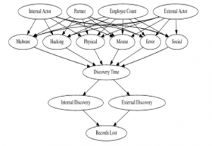
Figure 3. Causal Model for Cybersecurity (on VCDB)

3.4.  Data Breach Model

      Figure 3 represents the causal graph used as the basis for our causal analysis. The variables are all taken from VCDB and were decided on how accurately they could be mapped to a timeline of the data breach. Since all observational data given to us are all post-data breach, the way to approximate a causal effect for this analysis is to generate a model that shows a progression of events. Many of these variables and their sequencing were derived from personal interpretation than any logical standpoint. We will take a look at each variable type with their justifications.

• Actor
• Employee Count
• Action
• Discovery Time
• Discovery Method
• Records Lost

‘Actor’ is referring to the one who instigates the action against the victim. This could be a single person, a group of people, or even a natural disaster. In the causal model, the actor is spread amongst three categories: Internal, External, Partner. Internal actors are those who work within the company that is affected by the breach. External actors are those with no affiliation whatsoever with the company. Finally, partners do have or are part of an organization that has an affiliation with the company but are not from the company themselves. This variable represents a general categorizable description regarding the perpetrator of the data breach and is put near the top of the causal graph because the ‘actor’ is the one that will begin this data breach event.

‘Employee Count’ represents the general size of the victim company, which is represented by an integer value. Employee count was chosen as it is a variable that conveys a simple, but ordinal description of healthcare organizations.

Each of the types of data breaches (‘Malware’, ‘Hacking’, ‘Physical’, ‘Misuse’, ‘Error’, ‘Social’) are labeled as ‘Actions’ within VCDB. These are the treatment variables in which the analysis will be performed on. Each action is a binary state, and while there are a few rare cases that have multiple ‘Actions’ at once, these are still considered one data breach.

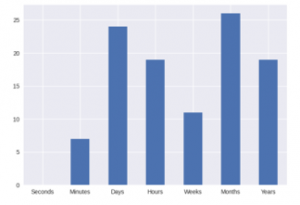
Figure 4. Distribution of ‘Discovery Time’

‘Discovery Time’ is the unit of time it took for the data breach to be discovered. VCDB does not have discovery time as an integer number. Instead, the variable is categorized as six different ranges of numbers, getting subsequently larger. Going under the assumption that the larger unit means that the actual discovery time was longer, the units were combined into one variable from 1-6, each representing a greater scale of time. The unit of time represents the general time frame of the data breach being discovered. Discovery time is one of the outcomes that is used to measure causality of data breaches. ‘Containment Time’ and ‘Exfiltration Time’ were considered as well. However, a high proportion of these entries remain unfilled in the VCDB dataset and are therefore not of much use.

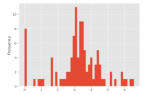
Figure 5. Distribution of Records Lost (log-scaled)

‘Discovery Method’ is the method by which the victim was first able to discover the data breach. Like ‘Actor’, this is also split into External, Internal, and Partner, which represents the relationship of the individual or group that discovered the breach to the victim company. External meant those unrelated to the company, Internal part of the company, and Partner are those affiliated with but not directly part of the company.

‘Records Lost’ is the second outcome we will be using as an outcome to test the causality of the causal model. Similar to Discovery Time, Records Lost is not an integer value, but ranges of values of subsequently greater number. This variable is also similarly combined into one variable ranging from 0-6. One major caveat is that this variable doesn’t have a defined unit and thus the scale of a unit of record is determined by each individual company. Part of the decision to focus on healthcare companies only was to mitigate this ambiguity.

4. Results and Analysis

Causal estimate calculations were run across all six ‘Actions’ (Social, Physical, Misuse, Malware, Hacking, and Error) and two outcomes (Discovery Time, Records Lost). This means multiple runs using the same causal model and dataset but changing the ‘Action’ and ‘Outcome’ input for each run until all permutations of each variable was covered. This was then repeated across all refutations. The causal estimate results for Propensity Score Matching on Discovery Time and Records Lost are shown in Figure 6 and 7, respectively.

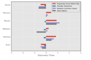
Figure 6. Causal Estimates for Discovery Time

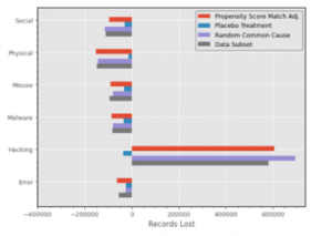
Figure 7. Causal Estimates of Records Lost

As seen in Figure 6 shows, the causal estimate of each action on Discovery Time shows quite a range of values and distributions across all actions. 3 actions (Physical, Misuse, Hacking) have positive causal estimates. indicating a potential strong causal relationship between the actions and lengthy discovery times. On the other hand, Social and Error turn out negative causal estimates, meaning that the impact of those two variables on discovery time is minimal. Lastly, Malware has a unique scenario where there is a split between the Propensity Score and its refuters.

For records lost (Figure 7), Hacking returns an overwhelming higher causal estimate compared to all other actions. In fact, all the other actions return a negative causal estimate. This does not necessarily mean the lack of causal effect of the other actions on records lost. However, it does provide strong indication that the greatest impact when it comes to records lost during a data breach is most likely the result of hacking as opposed to all other methods. Interestingly, this is backed up by both the Random Common Cause and Data Subset, but not the Placebo Refuter. In the Placebo case, the causal estimate returns a comparable negative value to the other actions. A possible explanation can be traced back to the nature of the dataset. While our causal model brings into consideration other causes of data breach, the distribution of the effect of each cause can be hard to separate. This is exacerbated when the Placebo Refuter randomizes the treatment variable, setting it so that every single entry in the dataset can also be considered part of the method of hacking.

This Placebo Refuter discrepancy is reflected across all the actions, which each return strongly diminished causal estimates. However, Hacking remains the only variable where the causal estimate goes from a positive to a negative value.

Another quirk to note is the large value of the causal estimate of Hacking on Records Lost. The reason for this exaggerated value is likely due to a lack of a solid control group within our data. The dataset provides us with a large selection of data breaches in a wide variety of companies. What the dataset lacks are scenarios where no data breach has occurred, generating an inherent bias within the dataset. This bias makes it so that the data do not fit well into linear regression, hence providing an overly large value as the result.

The most unexpected outcome was that propensity score stratification gave inconclusive results when ran on DoWhy, hence the lack of data on this portion of the analysis. After some analysis, we come to the conclusion that, due to the binary nature of each action, the distribution of the linear regression is not clear enough for stratification to be able to quantify and compartmentalize the dataset into groups. Hence, the resulting value outputs an inconclusive value due to a lack of substantial strata. This applies to stratification and not matching because matching disregards parts of the dataset with low propensity score; in stratification they still have an impact due to those data entries being assigned into strata.

Overall, in this specific scenario and dataset, Hacking would prove to be the most impactful amongst all methods of data breach.  However, the refuters give strong indication on where this impact is limited regarding not only the action itself but the dataset as a whole.

5. Conclusion and Future Work

The principal findings of this paper demonstrate the unique perspective of the causal modeling approach. Because we cannot realistically set up an experiment on data breach incidents, particularly in which all factors are readily provided, DoWhy and Causal Modeling allow us to simulate such experiments and make inferences with a degree of  robustness based on events that would otherwise be difficult to duplicate.

We identify a subset of factors in the Verizon Community Database and create a hypothesis based on the theory that malware and hacking are the most prominent causes of data breaches. Through propensity score matching and stratification, we measure the strength of the action behind data breaches. By running refutation tests, we are able to verify how well these metrics hold up, similar to how traditional experiments employ control groups or utilize a placebo treatment.

Ample room remains for the use of causal modeling in cybersecurity. We limit the scope of the factors considered in the Verizon Dataset to Actions in order to emphasize the results of the exploratory approach. A larger and denser dataset could utilize the causal model better.

Other fields of cybersecurity lend themselves well to causal modeling. In particular, the use of Directed Acyclic Graphs to model vectors of attack in a network intrusion scenario could lead to different approaches into how such cases are handled.

The study is important to the readers in the scientific community since it is relevant to formulating policies in industry and government, in order to avoid such problems in the near future. Given the context of the work, exhibited in the paper, our findings are worthy of note.

Conflict of Interest

The authors declare no conflict of interest.

Acknowledgments

We thank the Data Science Discovery Research Program of UC Berkeley and their participant, Rubina Aujla of UC Berkeley, 2018-2019, for contributions to causal modeling.

1.  P. Zornig, Probability Theory and Statistical Applications, De Gruyter. ISBN-13: 978-3110363197
2.  B. McLaughlin, On the Logic of Ordinary Conditionals, Buffalo, NY: SUNY Press, 1990.
3.  J. Pearl, Causality: Models, Reasoning, and Inference, Cambridge: Cambridge University Press, 2000.
4.  J. Pearl, Causality, 2nd edition, Cambridge University Press, 2009.
5. S. Thornley, R.J. Marshall, S. Wells, R. Jackson, “Using Directed Acyclic Graphs for Investigating Causal Paths for Cardiovascular Disease”, Journal of Biometrics & Biostatistics, 2013, 4:182. doi:10.4172/2155-6180.1000182
6. P. Menzies, H. Beebee. “Counterfactual theories of causation.”, 2001.
7. A. Chesher, A. Rosen, Counterfactual worlds. No. CWP22/15. Centre for Microdata Methods and Practice, Institute for Fiscal Studies, 2015.
8. A. Agresti, An Introduction to Categorical Data Analysis, 3rd Edition, Wiley Series in Probability and Statistics.
9. A. Sharma, E. Kıcıman,2020. Causal Inference and Counterfactual Reasoning. In7th ACM IKDD CoDS and 25th COMAD (CoDS COMAD2020), January 5–7, 2020, Hyderabad, India. ACM, New York, NY, USA,2 pages. https://doi.org/10.1145/3371158.3371231
10.  A. Sharma, E. Kiciman, et al. DoWhy: A Python package for causal inference. 2019.
11.  IBM Security 2019 Cost of a Data Breach Study: Global Overview
12. R. Anderson, 2001. Why Information Security is Hard-An Economic Perspective. In Proceedings of the 17th Annual Computer Security Applications Conference (ACSAC ’01). IEEE Computer Society, USA, 358.
13. Department of Health and Human Services, 2013. Modifications to the HIPAA Privacy, Security, Enforcement, and Breach Notification Rules Under the HITECH Act and the GINA Act; other Modifications to the HIPAA Rules (78 FR 5565), pp. 5565-5702
14.  VERIZON. Data Breach Investigations Reports Overview, 2019 (DBIR).

(Click Here)

(Click Here)