1. Introduction

The robotic arm is a programmable mechanical arm that works similar to a human arm. Robotic arms played a significant role in the process of industrial automation. The human-like dexterity of these robotic arms makes them efficacious in diverse applications in a variety of industries – manufacturing, atomic power plants, space exploration, material handling, painting, drilling, agriculture deployments [1], assistive robotics applications [2] and numerous other applications. The robotic arm typically comprises an end effector that is designed to manipulate and govern with the surroundings. The 6 DOF robot arm is designed to manipulate and govern with the surroundings. The 6 DOF is to pivot in 6 different ways that mimic a human arm. The major issues concerned in an industrial robotic arm are its mechanical structure and the control mechanism. The control mechanisms can be effectuated by 3 options: keyboard, joystick and slider-based control. Design of a lightweight robotic arm which can be compatible with any kind of robotic system. In the research, all the proffered control mechanisms adopted inverse kinematics, which makes it easier to control. The proposed control mechanisms are compatible with any other complex robotic systems of the same degrees of freedom. The dexterity of the robotic manipulator depends on the degree of freedom.

Kinematic analysis [3] is one of the important steps in the design of the robotic arm. The loop equations of complex robotic systems can be deduced from the kinematic equations. Joint angles regulate the motion of the robotic arm. Computer-Aided Design (CAD) software is the platform to create models with the given set of geometrical parameters. The proposed robotic arm was designed in Solid Works CAD software considering all the given sets of geometrical parameters. Robot Operating System (ROS) provides an integrated platform for the control of robotic systems. ROS is a special kind of framework initially developed with the purpose of working on robots in the research domains. In order to understand how the ROS framework works one should be clear about the concept of communication of messages through topic between nodes. Simulation is one of the ways to optimize the design and improve the control of robotic systems. ROS provides a 3-D visualizer (RVIZ) which helps in the visualization of the pose. With a properly-set URDF (Unified Robot Description Format) file, one can visualize the robot model in RVIZ. RVIZ is the simulation software used for the control of the 6-DOF robotic arm.

The design and development of 7-DOF arms [4] and even successful simulations on 11-DOF [5] arm are done by other authors with valid proofs of classic IK algorithms [6] in the discrete-time domain for robots. Taking those inputs into consideration the 6-DOF robotic arm in the paper was designed and tested with various goal positions using different modes of control. Algorithm developed for the keyboard based control [7] of the 6 DOF robotic arm using ROS which makes the control easier. The design and simulation of this robotic arm which is visualized in RVIZ. Simulation of a robot is also possible on the Gazebo platform [8] with the help of ROS_control packages and the generation of the robot conFigureuration is in Gazebo, it uses the URDF file and this is extensive use of a simulation platform for a real-life scenario. Simulation of the actuators in the arm can be done using various simulation software’s [9] like Matlab and Simulink [10], [11] but choosing RVIZ is preferable as there are many references to proceed. An open-source robot simulator called USARSim can also be used for both research and education of a robot’s general architecture [12]. An inverse kinematics algorithm [13] needs to be developed to achieve the goal positions in simulation over these platforms using the traditional method the DH parameter [11], [14] the inverse kinematics solutions [1], [15] for the arm have been derived. Few other authors used ADAMS [16] to simulate and evaluate the arm design but this paper deals with RVIZ simulation with multimode controls. With the help of ROS platform and MoveIt, the control [17] of the simulated arm was done and the three control modes [18] were tested. The sliding mode controller mechanism can be helpful for regulation of robotic arms with unknown behaviors [19]. Laser range method [20] can also be used for positioning and tracking tasks for a 6-DOF robotic arm. This method helps in the determination of the distance from the camera to the target. The workspace [21] of the arm and the path for reaching the goal position varies on the approach and techniques used while modelling the simulation. There are various other control mechanisms like trajectory tracking [22], master slave control [23], vibration control of a robotic arm with input constraints. Testing in real time doesn’t show accurate results due to backlash and electric issues. Considering this problem some authors proposed a self-learning algorithm [24] that uses positioning error after each trail. Simulation gives an idea about the performance of the algorithm, but in case if real time implementation performance changes due to several factors. One such thing is the connectivity and the architecture. Few authors explicitly gave intuition into the master-slave conFigureuration based tele existence    concept [25]. Considering all this leads, a 6 DOF robotic arm is simulated and tested by using different control mechanisms.

Contributions of the research is as follows:

• Kinematics based solution for the 6 DOF robotic arm is proposed.
• Validation of three control methodologies of the robotic arm.
• Simulation and evaluation of the 6 DOF robotic arm in RVIZ.

2. Architecture

The paper is primarily concerned about the different modes of control. Figure 1 represents the general architectural diagram which consists of control modes, a processing unit, and a 6 DOF robotic arm. ROS is used as the platform to develop software programs.

Control in testing the 6-DOF robotic arm by simulating it with an IK-based solution in RIVZ. The programs and files for the control modes and processing unit entirely return in CPP.

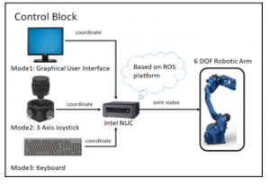
Figure 1:  General Architectural diagram.

2.1.  Control Block

The control block is the interface between the user and the robotic arm. It consists of three modes of control. The user can control a robotic arm using any of the below modes.

• GUI
• Joystick
• Keyboard

The robotic arms is equipped with a manipulator. A manipulator is a robotic gripper which is used to do dexterity. Figure 2 represents the software architecture of the 6 DOF robotic arm in the ROS platform.

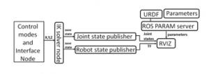
Figure 2: Software Architecture diagram.

The main aim is to control the robotic arm’s manipulator position in the RVIZ. Figure. 11, describes an RVIZ axis at the base of the robotic arm. The user can control the manipulator by using any of the control modes. These users input x, y, z coordinates will be published to IK solver node. The IK solver node will compute the joint states which are required for the manipulator to reach to the desired coordinates.

2.1.1 Control modes and Interface nodes

As there are different optional modes to command the robotic arm, interface node acts as an intermediate module that prioritizes the modes. The interface node will act as a bridge between the modes of control and the computing block IK_solver_node. The user can define the order of priority for the modes in the definition file in the interface module. On uploading the entire program, the compiler uses the updated definition file. On simultaneous publishing of data from the three control modes, always the highest priority mode values will be published to the IK_solver_node from the interface node.

2.1.2. IK Solver node

The Inverse Kinematics equations are generated by using Denavit-Hartenberg. An IK function is written in a computing file where it is passed with x, y, z parameters for computing. And there is a threshold evaluating block of code where the arms reach limit is checked whether it could reach the x, y, z coordinates. If the coordinate is present within the workspace of the arm it generates the individual joint values else, it generates the joint values which head to the maximum point it could reach in the direction heading to the input point. The generated joint values for the desired x, y, z coordinate point will be conveyed to the joint state publisher. Joint state publisher is the one which updates the joint values of the robotic arm simulation.

2.1.3. Graphical User Interface (GUI)

A user-friendly GUI was designed in QT Designer software [26] of version 4.8. Qt Designer is used to create user interface files containing windows and controls. Figure 3 depicts the representation of the graphical user interface which was developed in Qt Designer. The designed window consists of 3 fill in blocks, a SEND COORDINATES toggle button, a HOME toggle button, and a HALT toggle button.

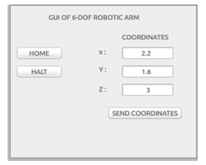
Figure 3: Representation of the graphical user interface.

The user can enter their x y z coordinates to which the user wanted the robotic arm to reach. On clicking the SEND COORDINATE button, the values will get published to the IK solver node. For resetting the robot, a HOME toggle button is designed. Whenever the user presses the toggle button, the robotic arm will reach the predefined pose. A HALT toggle button is also designed which will stop the motion of the robotic arm in case of emergency.

2.1.4. 3- Axis Joystick

The Joystick is another option for controlling the robotic arm. Figure 4 depicts a model of the 3-axes joystick. Arduino is the microcontroller used for taking the joystick values. The joystick will be connected to Arduino analog pins externally; through analog pins the joystick values are fetched.

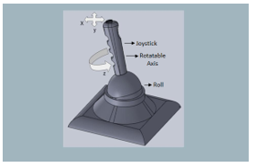
Figure 4: representation of 3 axes joystick

The three axes of the joystick are used to control the x y z coordinates position of the manipulator of 6 DOF robotic arm. If the user moves the joystick’s axis in forward direction, x value in the coordinate increases, similarly y and z can also be changed with the other two axes of the joystick. In this way, the user can control the manipulator position.

2.1.5. Keyboard

The keyboard is another mode of control. The keys ‘a’, ‘s’, ‘d’, ‘z’, ‘x’, ‘c’, ‘h’, ‘j’ are used to control the x, y, z values. When a key from ‘a’ or ‘s’ or ‘d’ on the keyboard is pressed, the x, y, z coordinate value increases respectively. When keys from ‘z’ or ‘x’ or ‘c’ are pressed then the coordinate variables x, y, z decreases respectively.  ‘h’ and ‘j’ are the home pose and halt buttons. These coordinates (x, y, z) are published to the interface node. And from the interface node to the IK solver node for further computation.

3. Design and Implementation

Robotic arms play a vital role in the industrial and social applications, where the design of the arm plays an important role in its function. According to the functionality, there are six main types of industrial robots: Cartesian, SCARA, cylindrical, delta, polar and vertically articulated. The design of the robotic arm that was developed for the research is not compromised in terms of the workspace. Any arm with revolute joints between all its base members falls in the category of the articulated robotic arm. An articulated arm has the ability to rotate all the joints (number of joints is from two to ten).  The reason behind the choice for the articulated robotic arm for the research is that it has more work envelope compared to SCARA, Delta, and Cylindrical.

Arm base is called the waist which is vertical to the ground and the upper body of the robot base is connected to the waist through a revolute joint which rotates along the axis of the waist and to which the second DOF (shoulder) is attached as similar to the arm in Figure 5. Third DOF which resembles the elbow of a human arm. The fourth DOF gives yaw movement, fifth gives the pitch and the last DOF gives the roll movement.  The 6-DOF articulated robotic arm was designed on Solid works and dimensions are mentioned in the Table 1. The first 3-DOFs give positional (i.e. x, y, and z) coordinates to the end-effector and the last 3-DOFs give the orientation of the end-effector. In the Table 1 base footprint is the base mounting stand for the robotic arm. The arm has 6 links namely base_link, Link1, Link2, Link3, Link4, Link5 and followed by the gripper. Link1 is the link between joints J1 and J2, Link2 is between joints J2 and J3. Similarly, for Link3, Link4, Link5 are the links with their respective joints.

Assembly file in Solid works is converted into a URDF file using Solid works with a maximum reach length of 1.248 m. Figure 5 and Figure 6 represents the design of the model of a 6-DOF robotic arm in Solid works. URDF is the conventional format for describing robots in ROS. The format is used to simulate a virtual arm. The joint positions, link lengths, and global origin are defined in the Solid works before exporting the assembly file of Solid works into URDF for simulation. The designed arm is simulated and controlled in Rviz using ROS. The evaluation of the designed URDF is done using MoveIt setup assistant which is ROS platform. In this section, the author first loaded the URDF file and created the collision matrix. MoveIt divides the arm joints and manipulators into groups, which helps to have a safer control of the robotic arm by resolving errors due to singularity issues.

Table 1: Joint link lengths.

i	joint	parent	child	Link length “(m)”	Shift in Origin “(m)”
0	Fixed base	Base footprint	base_link	0	0
1	J1	base_link	link1	0.15	0
2	J2	link1	link2	0.14	0
3	J3	link2	link3	0.45	0
4	J4	link3	link4	0.216	0.04
5	J5	link4	link5	0.091	0
6	J6	link5	link6	0.106	0.03
7	gripper	link6	Gripper  link	0.095	0
	Total			1.248

Figure 5. Front view of the Robotic arm

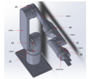
Figure 6. Top view of the Robotic arm

4. Robotic Arm Kinematics

The kinematics of the robotic arm are categorized into forward kinematics and Inverse kinematics. To calculate the kinematics solution the concepts of reference frames, Euler angles and Homogenous transforms are important.

4.1.  Reference Frame representation

Reference frames play an important role for the kinematics [27] of any arm. The general concept of reference frames is explained with the illustration in Figure 7. Consider point P, in the 2-D Cartesian as shown in Figure 7, is expressed with vector U relative to coordinate frame B. The same point P needs to be represented in frame A with vector V as shown in equations (1), (2) and (3). The matrix representation of the point P in frame A is given in (3). Any point in frame B is multiplied with  will project it onto frame A.

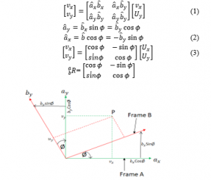
Figure 7: Reference frame representation of point P

4.2.  Euler angles

For a rigid body in space as shown in Figure 8 a box is considered as a rigid body, it has 3DOF for rotation those are roll, pitch, and yaw. These are called the Euler angles [28] and the representation of this rotational DOF. Euler angles are a system to describe a sequence or a composition of rotations. Conventionally, the movements about the three axes of rotations and their associated angles are described by the 3D rotation matrices. Equations (4), (5) and (6) show the matrix representation of roll, pitch, and yaw. These are 3D- rotation matrices and anticlockwise in direction.

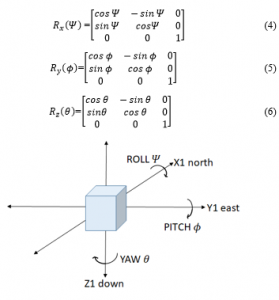
Figure 8: Euler angular representation for a rigid body

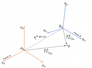
Figure 9: Relative frames for homogeneous transformation.

4.3.  Homogeneous transforms

Homogeneous transform is the representation of the transform matrix of one frame which is both rotated and translated with respect to some other unknown frame. In Figure 9 point in frame, B is transformed onto frame A. And the homogeneous transform is generated using rotational and translational matrices.

Equation (7) the term is the representation of point P vector with respect to frame A and this is 3*1 matrix. On the other end in the term  is the rotational matrix of frame B on to frame A and this is a 3*3 matrix.  Is the translation vector and this is 3*1 matrix. The  is a representation of point P vector with respect to B frame.

4.4.  Forward kinematics

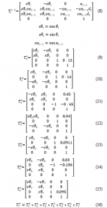
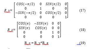
The forward kinematics [27] deals with location and pose of the end effector with the joint variables and parameters. Here the end-effector frame is mapped to the base joint of the arm using homogenous reference frames as discussed above. Denavit–Hartenberg parameters [14], [11] (also called DH parameters) are the four parameters associated with a particular convention for attaching reference frames to the links of a spatial kinematic chain, or robot manipulator. These are calculated for all the joints using the Figure 10 as a reference and data given in Table 2. Origin O(i) is the intersection between x(i) and z(i) axes. The joint angle (θ(i)) is t, the angle from axis x(i-1) to x(i) about z(i) using the right-hand rule. In joint 3 it has an offset of 180-degree constant between x (2) and x(3) and in joint 4 it has an offset of 90-degree constant between x(3) and x(4). Link twist (α(i-1)) is the angle from z(i-1) to z(i) measured about x(i-1) using right hand rule. In Table2 link length (a(i-1)) is equal to the difference between z(i-1) and z(i) along the x(i) direction. Link offset (d(i)) in Table 2 is the difference between x(i-1) and x(i) along the z(i) axis. Using equation 8, which is the general representation of the transform matrix from one frame to another. So by using the data available in Table 2 transform matrix for link 0 and link 1 is given in  in (8) Similarly, (9) is the transform for link 1 and link 2.  These are also similar kinds of transform matrices with their respective links. Finally, the transform matrix from base joint to the end effector is derived by shown in (16).  The orientation difference between the definitions of the gripper in URDF to the DH conventions so the rotation need to be done around y axis (17) and then need to be done around z axis (18) that is R_c shown in (19).

Table 2: DH-Parameters for the arm.

Links	O(i)	θ(i)	α(i-1)	a(i-1)	d(i)
0-1	1	θ1	0	0	0.15
1-2	2	θ2	-90	0	0.14
2-3	3	θ3+180	180	0.45	0.45
3-4	4	θ4+90	-90	0.04	0
4-5	5	θ5	-90	0	0.091
5-6	6	θ6	90	0.03	0.106
6-7	7	θ7	0	0	0.095

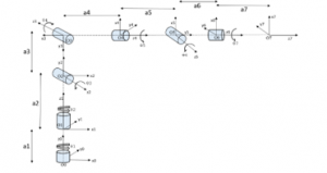
Figure 10: Cartesian representation of joints with rotational angles for    DH-parameters.

4.5.  Inverse kinematics (IK)

Inverse kinematics analysis is for obtaining the Joint angles by using end effector Cartesian space or position coordinates. Since the last three joints J4, J5, J6 in Figure5 and Figure 6 are revolute joints with joint axis intersection at J5 which would be wrist center (WC). Thus the kinematic of the IK is now evaluated by calculating Inverse position and Inverse Orientation.

4.5.1.   Inverse Position

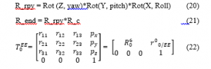
The inverse position problem is for obtaining the first three joint angles ( , , ). To evaluate Inverse Position the end effector position (Px, Py, Pz) and Orientation (Roll, Pitch, Yaw) need to be taken from the test case input data. Thus the rotation matrix for the end effector R_rpy shown (20). After the error correction the actual end effector rotation matrix R_end is given in (21). In (22) the obtained matrix  is the rotation part of the full homogeneous transform matrix  which is a transform matrix of end effector to the base joint. Using these concepts the joint angles ( , , ) are obtained.

4.5.2.         Inverse Orientation

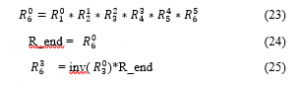
Inverse orientation problem is for obtaining the final three joint angles ( , , ).  The resultant transform is obtained using the individual DH transforms. Hence the resultant rotation is calculated as shown in (23). Since the overall the RPY (roll, pitch and yaw) rotation between base_link and gripper_link is equal to the product of individual rotations between the links as shown in (24). Multiply inverse matrix of  (inv( )) on either sides in (24) the resultant is shown in (25). The resultant matrix (25) on RHS (right hand side of the equation) does not have any variables after substituting the joint angles, and hence comparing LHS (left hand side of the equation) with RHS will result the equations for the last three joint angles ( , , ). Solving the obtained equations which results the joint angles.

5.  Experiment and results

The robotic arm in the research is designed for the manipulation tasks for various applications such as Coconut crop harvesting, Assistive robots like self-driving wheel chairs and Home robots, Search and Rescue robots for disastrous environments, Collaborative robots for research use and etc. The evaluation of the design and software was first done on RVIZ simulation with few goal positions, these goal positions are the most desired positions of the end effector during the general operations. Once the software simulation has given satisfactory results, the testing was done on hardware which was already built. The designed 6 DOF robotic arm is simulated in RVIZ.  An axis plugin has been added to visualize a coordinate axis at the base of the model robotic arm. The blue line indicates the z-axis, the red line indicates the x-axis and green line indicates the y-axis. The silver-coloured arm represents the goal pose of the arm for the user input values.

Figure 11 represents the different poses of the robotic arm when different coordinates are input to IK solver. Different x, y, and z coordinates are published to the interface module to manipulate the pose of the model arm. Table 3, 5 and 6 represents the outcomes of the IK solver when different goal points are input into the solver using different control methods on the RVIZ simulation platform. The output joint state values of all the goals positions in Figure 11 are given in Table 3, 5 and 6.  The input point is considered with respect to the RVIZ [17] world axis frame. With the IK based approach, the robotic arm was manipulated at the desired points in the RVIZ world frame simulation. The three control modes have been tested on 16 different goal positions. The input data from the interface block enters the IK solver node where the required joint values are calculated to achieve the respective input pose. These generated joint values are passed to Joint state publisher and robot state publisher where the required Tf and combined joint state array will be passed to the RVIZ for the simulation.

On comparing the accuracy between the three methods keyboard and GUI were able to position the arm to the desired goal pose. Joystick failed in some cases as the control mode was difficult to manipulate the robotic arm. Since the Joystick PWM values need to be transferred to ROS via a microcontroller, due to the disturbances in the hardware, in a few cases joystick input readings varied. There was 1%-3% error in the input and hence the output was also affected due to the change in the input values.  Comparing the results from Table 3, 4, 5 it is clear that GUI and Keyboard are two ideal methods to accurately position the robotic arm at a desired position.

The Figure 12 and Figure 13 illustrates the error percentage values while conducting a simulation experiment through a joystick.  A survey has been conducted by testing the system with a 20 number of individuals. Based on the outputs that were obtained, an analysis has been made on the error percentage in reaching the goal position. The error is calculated by comparing the correct outcomes obtained by an individual to the total no of test cases in Figure 12. And an analysis has been made which showed the error percentage for each goal pose. This is calculated based on the pass and fail cases obtained while conducting the survey by 20 individuals. The test results are plotted in Figure 13. Considering these errors, joystick control was avoided for the hardware test. The hardware test has been implemented using GUI as a control interface since the simulation results of keyboard based control and GUI based control are the same. Table 6 represents the outcomes of IK solver when implemented on hardware using GUI based control. It is observed that the output in the hardware testing using GUI based control is similar to the simulation testing using GUI.

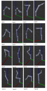
Figure 11:  The goal pose of the robotic arm on different user inputs.

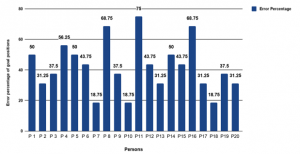
Figure 12: Error percentage for individual person

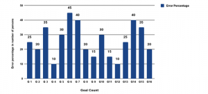
Figure 13 Error Percentage for individual goal position

Table 3: Outcomes of the joint state values from the IK solver node in simulation for the user input coordinates using GUI based control.

Goal Count	X position	Y position	Z position	DOF1 (radians)	DOF2 (radians)	DOF3 (radians)	DOF4 (radians)	DOF5 (radians)	DOF6 (radians)
Goal 1	0.301	0.651	0.525	1.2704	-0.9539	0.7554	-1.0660	1.3424	-1.185
Goal 2	0.402	0.730	0.376	1.0098	-1.222	0.9088	1.2786	0.476	1.4327
Goal 3	0.133	– 0.116	0.699	-0.5268	0.5868	-0.567	-0.6876	0.3067	0.0028
Goal 4	-0.392	0.532	0.825	2.2363	-0.6110	0.9545	0.043966	0.0151	0.6119
Goal 5	0.675	– 0.095	0.220	-0.0797	-1.0676	0.2312	-0.8217	0.4022	0.9090
Goal 6	– 0.019	0.242	1.020	1.4644	0.1755	0.3900	1.0424	0.5786	-1.297
Goal 7	0.204	0.644	0.529	1.3112	0.6556	0.3388	-0.9354	0.2892	1.14233
Goal 8	0.428	– 0.020	0.760	0	0	0	0	0	0
Goal 9	0.255	– 0.267	0.067	-0.89364	-1.23433	-0.70224	0.579329	0.924559	-0.41793
Goal 10	0.043	0.027	1.079	1.12537	0.424841	0.580440	-0.63930	0.2128	-0.99506
Goal11	– 0.017	– 0.110	0.759	1.396672	1.164312	-0.62972	0.222626	0.77854	0.505854
Goal 12	0.671	– 0.020	0.510	0.028259	-0.67949	0.223439	-0.42861	0.52486	0.095769
Goal 13	0.141	– 0.338	1.038	2.177904	0.639303	0.979159	1.05975	1.08808	-0.56990
Goal 14	0.281	– 0.123	0.844	2.831651	1.213924	-0.16744	0.57619	0.93674	-1.19414
Goal 15	0.303	– 0.716	0.108	-1.25223	-1.48647	0.71624	1.17593	0.725	-0.75893
Goal 16	-0.116	0.235	1.001	2.050420	0.0916879	0.3374000	0.156057999	1.03124	0.649038000

Table 4: Outcomes of the joint state values from the IK solver node in simulation for the user input coordinates using Keyboard.

Goal Count	X position	Y position	Z position	DOF1 (radians)	DOF2 (radians)	DOF3 (radians)	DOF4 (radians)	DOF5 (radians)	DOF6 (radians)
Goal 1	0.301	0.651	0.525	1.2704	-0.9539	0.7554	-1.0660	1.3424	-1.185
Goal 2	0.402	0.730	0.376	1.0098	-1.222	0.9088	1.2786	0.476	1.4327
Goal 3	0.133	– 0.116	0.699	-0.5268	0.5868	-0.567	-0.6876	0.3067	0.0028
Goal 4	-0.392	0.532	0.825	2.2363	-0.6110	0.9545	0.043966	0.0151	0.6119
Goal 5	0.675	– 0.095	0.220	-0.0797	-1.0676	0.2312	-0.8217	0.4022	0.9090
Goal 6	– 0.019	0.242	1.020	1.4644	0.1755	0.3900	1.0424	0.5786	-1.297
Goal 7	0.204	0.644	0.529	1.3112	0.6556	0.3388	-0.9354	0.2892	1.14233
Goal 8	0.428	– 0.020	0.760	0	0	0	0	0	0
Goal 9	0.255	– 0.267	0.067	-0.89364	-1.23433	-0.70224	0.579329	0.924559	-0.41793
Goal 10	0.043	0.027	1.079	1.12537	0.424841	0.580440	-0.63930	0.2128	-0.99506
Goal 11	– 0.017	– 0.110	0.759	1.396672	1.164312	-0.62972	0.222626	0.77854	0.505854
Goal 12	0.671	– 0.020	0.510	0.028259	-0.67949	0.223439	-0.42861	0.52486	0.095769
Goal 13	0.141	– 0.338	1.038	2.177904	0.639303	0.979159	1.05975	1.08808	-0.56990
Goal14	0.281	– 0.123	0.844	2.831651	1.213924	-0.16744	0.57619	0.93674	-1.19414
Goal 15	0.303	– 0.716	0.108	-1.25223	-1.48647	0.71624	1.17593	0.725	-0.75893
Goal16	-0.116	0.235	1.001	2.050420	0.0916879	0.3374000	0.156057999	1.03124	0.649038000

Table 5: Outcomes of the joint state values from the IK solver node in simulation for the user input coordinates using Joystick.

Goal Count	X position	Y position	Z position	DOF1 (radians)	DOF2 (radians)	DOF3 (radians)	DOF4 (radians)	DOF5 (radians)	DOF6 (radians)
Goal 1	0.305	0.652	0.525	1.2704	-0.9540	0.7556	-1.0660	1.3424	-1.185
Goal 2	0.406	0.7304	0.376	1.0098	-1.230	0.9089	1.2786	0.476	1.4327
Goal 3	0.135	– 0.116	0.699	-0.5268	0.5871	-0.567	-0.6876	0.3067	0.0028
Goal 4	-0.394	0.530	0.825	2.2363	-0.6116	0.9548	0.043966	0.0151	0.6119
Goal 5	0.67	– 0.095	0.220	-0.0797	-1.0681	0.2312	-0.8217	0.4022	0.9090
Goal 6	– 0.015	0.242	1.020	1.4644	0.1755	0.3900	1.0424	0.5786	-1.297
Goal 7	0.209	0.645	0.529	1.3112	0.6558	0.3389	-0.9354	0.2892	1.14233
Goal 8	0.421	– 0.020	0.760	0	0	0	0	0	0
Goal 9	0.255	– 0.267	0.067	-0.89364	-1.23433	-0.70224	0.579329	0.924559	-0.41793
Goal 10	0.043	0.028	1.079	1.12537	0.424841	0.58048	-0.63930	0.2128	-0.99506
Goal11	– 0.017	– 0.110	0.759	1.396672	1.164312	-0.62972	0.222626	0.77854	0.505854
Goal 12	0.671	– 0.020	0.510	0.028259	-0.67949	0.223439	-0.42861	0.52486	0.095769
Goal 13	0.141	– 0.338	1.038	2.177904	0.639303	0.979159	1.05975	1.08808	-0.56990
Goal14	0.281	– 0.123	0.844	2.831651	1.213924	-0.16744	0.57619	0.93674	-1.19414
Goal 15	0.303	– 0.716	0.108	-1.25223	-1.48647	0.71624	1.17593	0.725	-0.75893
Goal16	-0.116	0.234	1.001	2.050420	0.0916879	0.3375	0.156057999	1.03124	0.649038000

Table 6: Outcomes of the joint state values from the IK solver node on hardware testing for the user input coordinates using GUI

Goal Count	X position	Y position	Z position	DOF1 (radians)	DOF2 (radians)	DOF3 (radians)	DOF4 (radians)	DOF5 (radians)	DOF6 (radians)
Goal 1	0.301	0.651	0.525	1.2799	-0.9538	0.7600	-1.0659	1.3426	-1.184
Goal 2	0.402	0.730	0.376	1.0095	-1.222	0.9086	1.2786	0.480	1.4327
Goal 3	0.133	– 0.116	0.699	-0.5268	0.5868	-0.567	-0.6876	0.3067	0.0028
Goal 4	-0.392	0.532	0.825	2.2363	-0.611015	0.95467	0.0439666	0.01561	0.6119
Goal 5	0.675	– 0.095	0.220	-0.07978	-1.0676	0.2312	-0.82172	0.4022	0.9090
Goal 6	– 0.019	0.242	1.020	1.464454	0.1755	0.3900	1.0424	0.57862	-1.29711
Goal 7	0.204	0.644	0.529	1.3112	0.6556	0.3388	-0.9354	0.2892	1.14233
Goal 8	0.428	– 0.020	0.760	0	0.	0	0	0	0
Goal 9	0.255	– 0.267	0.067	-0.89364	-1.234335	-0.702246	0.579329	0.924559	-0.41793
Goal 10	0.043	0.027	1.079	1.12537	0.424841	0.5804405	-0.63930	0.21285	-0.99506
Goal11	– 0.017	– 0.110	0.759	1.3966725	1.1643121	-0.629728	0.2226262	0.77854	0.505854
Goal 12	0.671	– 0.020	0.510	0.028259	-0.67949	0.223439	-0.42861	0.52486	0.095769
Goal 13	0.141	– 0.338	1.038	2.177904	0.639303	0.97915954	1.0597566	1.088084	-0.56990
Goal14	0.281	– 0.123	0.844	2.831651	1.2139244	-0.16744	0.576198	0.93674	-1.19414584
Goal 15	0.303	– 0.716	0.108	-1.252234	-1.48647	0.7162445	1.175932	0.72512	-0.75893
Goal 16	-0.116	0.235	1.001	2.050420	0.0916879	0.3374000	0.156057999	1.03124	0.649038000

6. Conclusion

In this research work, the authors proposed and evaluated reliable methods for controlling a robotic arm by testing it in both hardware and simulation using RVIZ. The authors in [17] used the MoveIt to build a kinematics library for the IK of the robotic arm, but as an extension of that, this research designed and developed a kinematics-based solution using DH parameters method. Using the derived equations, successfully tested the designed robotic arm in Rviz using the proposed control mechanisms. A survey is conducted in evaluating the best control methodology where Figure [12] and Figure [13] depict the results. Based on the survey, the research validates that the joystick failed in achieving the desired input coordinate positions due to signaling and hardware issues. But GUI and Keyboard showed better results in controlling the arm.

As a rule, simulations do not reproduce the exact real-time behavior of an entity or a system. PID based control can reduce the error. The research can be enhanced by testing the proposed design in the Gazebo simulation software. Gazebo provides the flexibility to use a PID-based controller, which helps in smooth and exact mimicking of the real-time robotic arm as per simulation in RVIZ. The proposed testing gives the developer good results. Design of the end effector can be improved for performance of multiple, divergent tasks in a real time environment. The singularity issues can be reduced for better performance and enhancement of the task.

Acknowledgment

We are grateful for Amrita Vishwa Vidyapeetham and Humanitarian and Technology Labs for providing us with all the sophisticated requirements to develop and complete this paper.

1. Megalingam R.K, Sivanantham V, Kumar K.S, Ghanta S, Teja P.S, Gangireddy R, Sakti Prasad K.M, Gedela V.V, “Design and development of inverse kinematic based 6 DOF robotic arm using ROS”, International Journal of Pure and Applied Mathematics, 118, pp. 2597-2603, ISSN: 1314-3395
2. Xinquan Liang, Haris Cheong, Yi Sun, Jin Guo, Chee Kong Chui, Chen-Hua Yeo, “Design, Characterization, and Implementation of a Two-DOF Fabric-Based Soft Robotic Arm”, IEEE Robotics and Automation letters(Volume:3,Issue:3,July2018),https://doi.org/1109/LRA.2018.2831723
3. Asghar Khan, Wang Li Quan. “Structure design and workspace calculation of 6-DOF underwater manipulator”. 2017 14th International Bhurban Conference on Applied Sciences and Technology (IBCAST), 10-14 Jan 2014, https://doi.org/ 10.1109/IBCAST.2017.7868119
4. Elkin Yesid Veslin; Max Suell Dutra; Omar Lengerke; Edith Alejandra Carreño; Magda Judith Morales, “A Hybrid Solution for the Inverse Kinematic on a Seven DOF Robotic Manipulator”, IEEE Latin America Transactions ( Volume: 12, Issue: 2, March 2014 ), https://doi.org/1109/TLA.2014.6749540
5. Pietro Falco; Ciro Natal, “On the Stability of Closed-Loop Inverse Kinematics Algorithms for Redundant Robots”, 05 May 2011, IEEE Transactions on Robotics (Volume: 27, Issue: 4, Aug. 2011 ),https://doi.org/1109/TRO.2011.2135210
6. Seo-Wook Park, Jun-Ho Oh, “Hardware Realization of Inverse Kinematics for Robot Manipulators”, IEEE Transactions on Industrial Electronics Vol.41, No 1, February 1994, https://doi.org/1109/41.281607
7. Rajesh Kannan Megalingam, Nigam Katta, Raviteja Geesala, Prasant Kumar Yadav, “Keyboard Based Control and Simulation of 6 DOF Robotic Arm using ROS”, 2018 4^th International Conference on Computing Communication and Automation(ICCCA), https://doi.org/10.1109/CCAA.2018.8777568
8. Wei Qian, Ziyang Xia, Jing Xiong, Yangzhou Gan, Yangchow Guo, Shaokui Weng, Hao Deng, Ying Hu, Jiawei Zhang, “Manipulation Task simulation using ROS and Gazebo”, Robotics and Biomimetics (ROBIO), 2014 IEEE International Conference”, https://doi.org/1109/ROBIO.2014.7090732
9. Žlajpah Leon, Simulation in robotics (2008) Mathematics and Computers in Simulation, 79 (4), 15 December 2008, pp. 879-897, https://doi.org/10.1016/j.matcom.2008.02.017
10. Kichang Lee ; Jiyoung Lee ; Bungchul Woo ; Jeongwook Lee ; Young-Jin Lee, Kimhae-si ; Syungkwon Ra “Modeling and Control of an Articulated Robot Arm with Embedded Joint Actuators ”,2018 International Conference on Information and Communication Technology Robotics (ICT-ROBOT), https://doi.org/1109/ICT-ROBOT.2018.8549903
11. Alla N Barakat, Khaled A. Gouda, Kenza.Bozed, “ Kinematics analysis and simulation of a robotic arm using MATLAB”,2016 4th International Conference on Control Engineering & Information Technology (CEIT),16-18 Dec. 2016, Hammamet, Tunisia, https://doi.org/ 10.1109/CEIT.2016.7929032
12. Stefano Carpin, Mike Lewis, Jijun Wang, “USARSim: a robot simulator for research and education” Proceedings 2007 IEEE International Conference on Robotics and Automation, 10-14 April 2007, Roma Italy, https://doi.org/ 10.1109/ROBOT.2007.363180
13. ] Jun-Di Sun; Guang-Zhong Cao; Wen-Bo Li; Yu-Xin Liang; Su-Dan Huang, “Analytical inverse kinematic solution using the D-H method for a 6-DOF robot”, 2017 14th International Conference on Ubiquitous Robots and Ambient Intelligence (URAI), https://doi.org/10.1109/URAI.2017.7992807
14. Akhilesh Kumar Mishra; Oscar Meruvia-Pastor; “ Robot arm manipulation using depth-sensing cameras and inverse kinematics ”2014 Oceans-St John’s,14-19 September 2014 IEEE International Conference, St. John’s, NL, Canada, https://doi.org/1109/OCEANS.2014.7003029
15. A. G. Gutiérrez; J. R. Reséndiz; J. D. M. Santibáñez; G. M. Bobadilla, “A Model and Simulation of a Five-Degree-of-Freedom Robotic Arm for Mechatronic Courses”, IEEE Latin America Transactions ( Volume: 12, Issue: 2, March 2014 ) ,https://doi.org/ 10.1109/TLA.2014.6749521
16. Zenghua Bian ; Zhengmao Ye ; Weilei Mu,” Kinematic analysis and simulation of 6-DOF industrial robot capable of picking up die-casting products”, 2016 IEEE International Conference on Aircraft Utility Systems (AUS), https://doi.org/ 10.1109/AUS.2016.7748017
17. Hernandez-Mendez, C. Maldonado-Mendez, A. Marin-Hernandez, H. V. Rios-Figureueroa, H. Vazquez-Leal and E. R. Palacios-Hernandez, “Design and implementation of a robotic arm using ROS and MoveIt!”, 2017 IEEE International Autumn Meeting on Power, Electronics and Computing (ROPEC), Ixtapa, 2017, pp. 1-6, http://doi.org/ 10.1109/ROPEC.2017.8261666
18. Weimin Shen, Jason Gu, Yide Ma, “3D Kinematic Simulation for PA10-7C Robot Arm Based on VRML”, 18-21 Aug. 2007, Jinan, China. https://doi.org/10.1109/ICAL.2007.4338637
19. José de Jesús Rubio, “Sliding mode control of robotic arms with dead zone”, IET Control Theory & Applications (Volume: 11, Issue: 8, 5 12 2017), https://doi.org/1049/iet-cta.2016.0306
20. Megalingam R.K, Rajesh Gangireddy, Gone Sriteja, Ashwin Kashyap, Apuroop Sai Ganesh “Adding intelligence to the robotic coconut tree climber” 2017 International Conference on Inventive Computing and Informatics (ICICI), 23-24 Nov. 2017, Coimbatore India, https://doi.org/1109/ICICI.2017.8365206
21. Teerawat Thepmanee, Jettiya Sripituk, Prapart Ukakimapurn, “A simple technique to modeling and simulation four-axe robot-arm control” 17-20 Oct. 2007, Coex, Seoul, Korea, https://doi.org/1109/ICCAS.2007.4406694
22. Tingting Meng; Wei He, “Iterative Learning Control of a Robotic Arm Experiment Platform with Input Constraint”, IEEE Transactions on Industrial Electronics (Volume: 65, Issue: 1, Jan. 2018), https://doi.org/1109/TIE.2017.2719598
23. Gourab Sen Gupta, Subhas Chandra Mukhopadhyay, Christopher H. Messom, Serge N. Demidenko, “Master-Slave Control of a Teleoperated Anthropomorphic Robotic Arm With Gripping Force Sensing ”, IEEE Transactions on Instrumentation and Measurement ( Volume: 55, Issue: 6, Dec. 2006 ),https://doi.org/1109/TIM.2006.884393
24. Lucibello,“ Repositioning control of robotic arms by learning ”, IEEE Transactions on Automatic Control ( Volume: 39, Issue: 8, Aug 1994 ), https://doi.org/ 10.1109/9.310053
25. Qingyuan Sun; Lingcheng Kong; Zhihua Zhang; Tao Mei, “Design of wireless sensor network node monitoring interface based on Qt”, 2010 International Conference on Future Information Technology and Management Engineering, Changzhou, 2010, pp. 127-130
26. Takuma; Y. Asahara ; H. Kajimoto ; N. Kawakami ; S. Tachi, “Development of anthropomorphic multi-D.O.F master-slave arm for mutual telexistence ”, IEEE Transactions on Visualization and Computer Graphics ( Volume: 11 , Issue: 6 , Nov.-Dec. 2005 ), https://doi.org/ 10.1109/TVCG.2005.99
27. Ramesh, S. B. Hussain and F. Kangal, “Design of a 3 DOF robotic arm,” 2016 Sixth International Conference on Innovative Computing Technology (INTECH), Dublin, 2016, pp. 145-149, https://doi.org/1109/INTECH.2016.7845007
28. Jose de Jesus Rubio; Adrian Gustavo Bravo; Jaime Pacheco; Carlos Aguilar,“Passivity analysis and modeling of robotic arms”, IEEE Latin America Transactions ( Volume: 12 , Issue: 8 , Dec. 2014 ) ,https://doi.org/1109/TLA.2014.7014505

(Click Here)

(Click Here)