1. Introduction

The amount of data has proliferated every day, which strengthened the need for a high-speed database management system. With the current amount of data that big, very powerful processing powers need also increased. On the other hand, real-time data processing needs have pushed the conventional database into its limits. Digital Universe & EMC estimates that data collected in 2020 will have nearly 44 trillion gigabytes. This situation stimulates the born of another database system such as Hadoop system, Big Query, Apache Spark, ClickHouse, Amazon Athena, etc. All of these databases are born with enormous processing power which makes big data processing much faster. However, their processing capabilities depend on the number of nodes and parallelism of the current CPU device, which mean this leads to increased power consumption [2, 3].

In 2013, there is a new database created which gets the attention of some researchers, this kind of database is using graphics processing units (GPUs) to help central processing unit (CPU) on processing the data which makes it very powerful but in an affordable way. The name of this new database is OmniSci. GPU is very famous for its parallel processing [4]. However, due to different be transferred into GPU memory to do data processing on GPU [5]. The data transfer between GPU device and main memory is going through PCI Express bus slot, Nowadays, the latest PCI Express bus on the market is version 5.0 which have a maximum transfer speed of 63.02 GB/s, this behaviour caused the huge processing amount of data on GPU will have I/O bottleneck. Some researchers found the side effect of using GPU as a co-processor which can make a query run slower than CPU only processing. The main challenge of doing data processing on GPU is the data transmission bottleneck while doing non-numerical type data processing [6]. Hence, the query execution time using GPU co-processor not guarantee the processing will be faster compared to the CPU only. Until today, We cannot find research that fully identifies the components of query which still not optimized on the GPU nor use a machine learning model to switch query execution platform between CPU and GPU in a hybrid way.

In this research, we introduce a hybrid approach to select the optimum execution platform processing platform between CPU and GPU with a machine learning model helps. The main focus of this research is to find out which query is faster on CPU and which on GPU co-process, to do that, we will create an automatic query parser to parse a single query to determine machine learning parameters, and based on obtained parameters, the machine learning model will determine which platform is the best to execute the parsed query. By do query processing platform management, we can also manage the usage of GPU memory to ensure a GPU type query can be executed on GPU.

2. Background & Related Works

2.1        GPU Architecture

GPU is a device that commonly used on a computer or notebook. GPU’s primary purpose is to do intensive graphical functions such as watching videos, gaming, or video rendering. As the time being, GPU was started to be used as general-purpose processing [7]. GPU become very popular on general-purpose processing due to its Single Instruction Multiple Data (SIMD) characteristics which will help to boost processing performance on data-intensive computations [5, 8]. However, apart from its processing power, there is a challenge that needs to be faced while utilizing the GPU processor as a CPU co-processor due to its memory architecture.

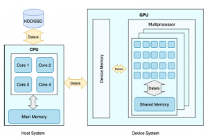
Figure 1: CPU – GPU Architecture [9]

As shown on Figure 1, GPU usually called as a device system, while CPU is called as a host system, the device system is connected to the host system using PCI express bus. Each host and device has its own memory and processors, typically the host and device memory do not share the same address space, which means the device system cannot directly access the host’s memory and vice versa. Therefore, to do data processing on GPU, the data need to be transferred into the device memory first. In general, data are stored on a hard drive or solid-state drive, this resulting the data need to pass through host memory then device memory and after the device has finished on processing the data, it will send the data back to host memory in order to show the data to the users [9]. Due to these I/O procedures, the GPU will not help much to improve the processing speed if there is an I/O bottleneck on the system [10].

2.2        OmniSci

When first released, OmniSci is named as Mapd, OmniSci is an open-source SQL-based, relational and columnar type of database which developed to leverage the data processing needs nowadays by utilizing the use of GPU processing power. Its ability to outperform the current big data platform makes it popular to be an alternative solution for big data processing.

A vital component of the OmniSci SQL engine performance advantage is the hybrid or parallelized execution of queries. A parallelized code allows a processor to compute multiple data items simultaneously. This is necessary to achieve optimal performance on GPU, which contains thousands of execution units.

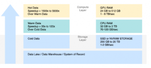
Figure 2: OmniSci Advanced Memory Management [11]

Figure 2 shows that OmniSci has advanced memory management with three-tier caching in their system. The caching contains two layers of computation, storage layer, and compute layer. On the storage layer, it is started with the data itself. The data can be sourced from various sources, i.e. data lake, data warehouse, or system of records, then continue to the third tier of caching called cold data, in this tier the data will be cached on SSD or NVRAM Storage. Moving to the compute layer, there lay second-tier caching called warm data, in this tier the caching will happens in host memory, or usually, we call it RAM, and the first tier called warm data where the caching is happens on the device memory. All three tiers meant to eliminate the transfer overhead between CPU and GPU.

During the query execution, OmniSci system adapts query vectorization and hybrid execution system. This feature allows the system to vectorize the code and compute multiple data items simultaneously across multiple GPUs and CPUs [11].

2.3        Scikit-learn

For machine learning, this paper will use help from Scikit-learn, Scikit-learn is a python framework which provides many popular machine learning algorithm implementations. It is easy to use interface, and well-integrated with python language make this framework can easily be used by data analysis who not specialized in the software and web industries [12]. In this paper, we will test our model using Random Forest, Nave Bayes, Logistic Regression, KNN, and Adaptive Boosting classifier algorithm.

2.3.1       Random Forest

Random Forest is an ensemble machine learning algorithm that can be used to do data classification and regression. Random Forest is prevalent due to its excellent performance on many data sets. In many cases, Random Forest achieved the best in class performance with higher accuracy than another machine learning algorithm [13, 14], hence we wanted to try this machine learning algorithm with our model to see how it performs.

2.3.2       Nave Bayes

Nave Bayes classification is a straightforward probabilistic model. The model is based on Bayes rule along with a robust assumption of independence. The main characteristic of the Nave Bayes Classifier is a powerful assumption (naive) of independence from each condition or event. The advantage of using Nave Bayes method is that it only requires a small amount of training data to determine the estimated parameters needed in the classification process, and words are conditionally independent of each other. As the drawback, this assumption will slightly affect the accuracy of text classification. However, as an advantage, it will make the high-speed classification algorithm applicable to the problem [15, 16]. Nave Bayes characteristics are matched with what we are looking for in this paper, which is a high-speed classification machine learning algorithm with the highest accuracy.

2.3.3       Logistic Regression

Logistic Regression is a technique that can be used for traditional statistics as well as machine learning. Logistic Regression will work by predicts if something is true or false, 0 and 1, or Yes and No. Logistic Regression is widely used on some classification tasks due to its simplicity and lightweight, and it does not need many computational resources to operate. We choose this algorithm to test with is because it fits our model, whereas there is only two decision that needs to be made, CPU or GPU [16, 17].

2.3.4       K-Nearest Neighbor

K-Nearest Neighbour is a supervised learning algorithm where the result of a new instance classified based on the majority of the nearest K-neighbor category. KNN become popular among classifier algorithms is because of its simplicity, practical, robust, and conceptual clarity. It also can achieve higher accuracy on unknown or non-normal distributed data set [18]. We are choosing KNN as one of 5 machine learning algorithms we test in this paper is because it can perform well in unknown or non-normal distributed data sets, which will fit on our model where usually most user’s ad-hoc query is non-predictable.

2.3.5       Adaptive Boosting

Adaptive boosting or in short AdaBoost is a machine learning algorithm introduced in 1995 by Freud and Schapire. The advantage of this algorithm is it fast, simple, and easy to program due to there is only one parameter that needs to be tuned which is the number of rounds [14, 19].

2.4        TPC-H Dataset & Query set

The TPC Benchmark H (TPC-H) is a benchmark dataset for a decision support system. The queries and information provided by TPC-H were selected to make the dataset can have excellent relevance with the industry-wide but in ease of implement manner. TPC-H dataset size can freely be customized based on the user’s needs. TPC-H also contains query set for system testing; the query set consist of 22 query type with various complexity. As shown on Figure 3, TPC-H has eight tables, and every relation for each table is one to many relationship[20].

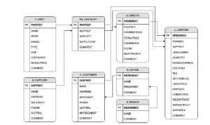
Figure 3: TPC-H Schema [11]

2.5        Related Works

The research on GPU processing sector started in 2004, in this year [21] do research to create graphics card as a co-processor to do data processing. In their research, they focus on speeding up basic database queries such as select and aggregation and got 108x speedup over CPU. This research got more attention from other researchers to continue to investigate the possibility to create a fully operational GPU database. The research on this sector is continued by [4]; they create and implement the use of GPU processing power to SQLite. In their research, they demonstrate the main principle of the GPU database that data processing efficiency on a GPU card depends on the I/O cost. They explain that GPU cannot help to increase the data processing performance if the data need to be processed from physical hard drive due to I/O limitation from hard drive to GPU. This research got 35x speedup over CPU. This research then also continued by [22] by enhancing the Bakkum model to be able to do a Relational database join by translate SQL code into opcode, and as a result, they get 20 to 30 processing times speedup over the CPU processing time.

In 2011, [10] did research on the data transfer between main memory to GPU memory; they explain even though GPU can do a very vast data processing, we also need to pay attention to the transfer time between main memory to GPU. If the transfer time overshadowing the processing time, there will be no speedup obtained from GPU. Hence, they suggest on PCI-Express port usage.

Another research done by [23], they recommend the use of column-major storage is very recommended to maintain the data transfer between host memory and device memory. In their research, they also found that the efficiency of data processing on GPU will depend on the amount of data that will be processed. In the case of small data, the CPU will be the best platform to process the data.

[1] In 2016 conduct an experiment to test GPU as a query accelerator, they are testing geospatial data computation on GPU with help from Mi-Galactica as a GPU accelerator. As the results, they found if the framework execution time is outperforming the Spark one, and they state that GPU based data processing can be an alternative to Big Data.

In 2017, [6] trying to find the problem of GPU speedup which hugely depends on the amount of data processed by creating an algorithm to make a hybrid approach to select the processing platform between CPU and GPU. They call the algorithm as Hybrid Query Processing algorithm.

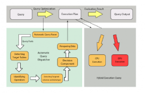
Figure 4: Related Work Framework [6]

As shown in Figure 4, the algorithm works by splitting 1 query into subquery block, from this block system will identify which operator being used, what the data type, how big the data and the aggregation type, then the system will do speed comparison to see which platform complete the query faster. However, in this algorithm, the data used to compare the speed is only a sample of 10 top rows which might not represent all rows in the table.

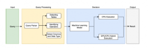
Figure 5: Proposed Framework

3. Proposed framework

In this section, we discuss the detail of the proposed framework. Figure 5 show the overall of the proposed framework. There are four main sections: input, Query Processing, Decision, and Output. The process started by query inputted into the system, then the system will process any inputted query by split the query and extract the information from it. The extracted information then will be pass to the machine learning model, which has a crucial role to determine which platform will be used to run the query. Finally, the system will show the query result in the output section.

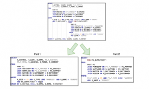
Figure 6: Sub Query Split Illustration

3.1        Query parser

After queries are submitted, the system will process the query by parsing it into several parts and extract the information. Query parser part is the most crucial part of the framework because if the system cannot identify a query correctly, the result accuracy will also not be convinced. To do that, we need to identify if there are any subqueries or not. Figure 6 show a scenario where subqueries exist on a query. In this scenario, the system will split the query into two parts, the main query, and the subqueries.

After the query become several parts, the system then will identify query components from each part of inputted queries starting from the number of columns, aggregation type, number of joins, join type, number of filters, number of wild cards, having filter, and group by and order by columns. Finally, the system will merge the analyzing result of each part of the query then pass it into machine learning.

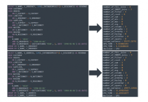
Figure 7: Identical Feature Generated Sample

In some scenarios illustrated in Figure 7, we found that the query parser result might generate some same result while the selected columns are different. The difference between 2 queries on Figure 7 is only on the column selection. The first query is selecting L ORDERKEY while the bottom query is selecting S ADDRESS, but the execution result is showing the bottom query runs faster on GPU co-processor.

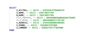
Figure 8: Column to ASCII Conversion Illustration

To overcome this kind of situation, we make the system identify the uniqueness of the selected column by converting the selected column into ASCII number, as shown in Figure 8.

The number then will be summed up and converted into a 5-digit float, i.e., 30873177894140434 will become 30873.177894140434. By using this method, we can get a unique feature combination of the generated data. The real calculation result is shown in Figure 7 on the column variance feature, while the number of column feature is the same, but the ASCII calculation is showing different results.

3.2        Machine Learning Model Methodology

The machine learning model is the second most crucial part of the framework. This part will become the brain of the framework, which will decide the best query execution platform for each inputted query. As illustrated on Figure 9 The machine learning model will work after the system has successfully extract information from the inputted query. The extracted queries become dataset. 75% of the dataset will be sent to the machine learning model to train the model, while another 25% of the dataset will be sent to the trained machine learning model to decide which platform will be selected to run the query.

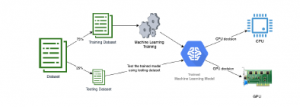
Figure 9: Machine Learning Methodology

For machine learning algorithms itself, we are testing five machine learning algorithms, Random Forest, Nave Bayes, logistic Regression, KNN, and adaptive boost classifier module from scikitlearn. The reason we choose these five machine learning algorithms is due to their simplicity, effectiveness, robustness, and performance reputation on doing the classification. Out of five algorithms, we will choose a machine learning which has the least testing time and high accuracy. Hence the machine learning decision timing will not overshadow the query processing time itself. The machine learning model will make a decision based on the inputted parameters listed in Table 1. These parameters were chosen based on the previous paper [6].

3.3        Generate Training Data

To make machine learning model can effectively select the best platform to run a query, the machine learning need to be trained first. To train the machine learning, we need to create a dataset which will be inputted into the machine learning model and become its knowledge.

To create a dataset, we use the TPC-H queries test set as a base and use a binary model to generate alternatives query. The TPC-H queries test set contains 22 queries, and after using a binary model to generate alternative for each query type, it contains 3365 queries as shown in Table 2.

This binary model was created to make the system can cover all query possibilities which usually user use, the binary model as described in Figure 10.

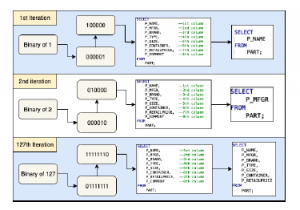
Figure 10: Query Generation Example

Table 2: Total Number of Generated Dataset

Row Labels	CPU	GPU	Total
Type 1	3	5	8
Type 2	254	0	254
Type 3	68	443	511
Type 4	0	14	14
Type 5	164	90	254
Type 6	1	15	16
Type 7	503	8	511
Type 8	511	0	511
Type 9	24	6	30
Type 10	6	219	225
Type 11	30	0	30
Type 12	0	30	30
Type 13	0	12	12
Type 14	1	127	128
Type 15	0	14	14
Type 16	14	0	14
Type 17	2	126	128
Type 18	2	508	510
Type 19	21	107	128
Type 20	0	15	15
Type 21	0	15	15
Type 22	7	0	7
Grand Total	1611	1754	3365

The binary model will work to generate the column selection, grouping and sorting. While for the table name, relation, and aggregation will be determined based on the TPC-H query set. After the query set has been generated, the queries will be run on GPU and CPU sequentially to get the GPU TIME and CPU TIME information. The result then will be used to determine the label on each query. The query labelling will use the following rules:

• CPU TIME > (GPU TIME-GPU TIME REBATE) -> GPU

Execution

• CPU TIME ≤ (GPU TIME-GPU TIME REBATE) -> CPU

Execution

On the GPU there is a variable called GPU TIME REBATE, this variable is defined to give advantage for CPU, in this paper we give GPU TIME REBATE value of 0.5 seconds. This value may be variable depends on each user’s tolerance. We give CPU advantage due to during our experiment is because we found that many queries have almost similar execution time for both CPU and GPU. Meanwhile, GPU memory was considered more expensive than host memory, therefore if a query runs on GPU but there is no much time gained over CPU, it will be waste of GPU memory, the OmniSci was using caching in their system, and if there is no enough GPU memory for a query to be executed on GPU, those queries will be passed to host system to be processed using CPU. In this case, if the GPU memory was full because of a query that did not have much gain over CPU while there is a query which will have more time gain over CPU need to be executed on GPU but failure due to memory is full, it will be very unfortunate.

3.4        Machine learning model Training

Table 1: Extracted Feature Feature Data Type Description NUMBER OF JOINS Integer Showing total number of joins NUMBER OF LEFT JOINS Integer Showing number of left joins NUMBER OF INNER JOINS Integer Showing number of inner joins NUMBER OF FILTER Integer Showing number of filters NUMBER OF COUNT Integer Showing number of count NUMBER OF SUM Integer Showing number of sum NUMBER OF MIN Integer Showing number of min NUMBER OF AVG Integer Showing number of avg NUMBER OF COLUMN Integer Showing number of columns NUMBER OF GROUPBY Integer Showing number of groupby NUMBER OF ORDERBY Integer Showing number of orderby NUMBER OF HAVING Integer Showing number of having NUMBER OF WILDCARD Integer Showing number of wildcards NUMBER OF SQUERY Integer Showing Number of Sub Queries COLUMN VARIANCE Float Result of ASCII value from selected column GPU TIME Float Showing GPU execution time CPU TIME Float Showing CPU execution time DECISION varchar (3) Showing label for machine learning

To train the machine learning model, the dataset will be split into a training set and test set with 75 – 25 ratio, 75 % used to train the model, and 25 % used to validate. As shown in Table 3 for machine learning able to cover all query scenarios, the data is divided on the query type level. To validate the results, we also use cross-validation with amounts of 5 folds.

Table 3: Training and Test data Split Result

Row Labels	Total	Training	Test
Type 1	8	6	2
Type 2	254	190	64
Type 3	511	383	128
Type 4	14	10	4
Type 5	254	190	64
Type 6	16	12	4
Type 7	511	383	128
Type 8	511	383	128
Type 9	30	22	8
Type 10	225	168	57
Type 11	30	22	8
Type 12	30	22	8
Type 13	12	9	3
Type 14	128	96	32
Type 15	14	10	4
Type 16	14	10	4
Type 17	128	96	32
Type 18	510	382	128
Type 19	128	96	32
Type 20	15	11	4
Type 21	15	11	4
Type 22	7	5	2
Grand Total	3365	2517	848

4. Experimental Evaluation

4.1        Experimental Setup

The proposed approach has been conducted on a PC with Core i7 3770 processor, 16gb of Ram, Nvidia GTX 970 with 4gb GDDR5 memory. The running OS is Ubuntu 18.04 with CUDA 10, on the software side, we are using scikit-learn version 0.21.3, OmniSci 4.7, and the code is written under python 3 languages. For the database setup, we are using JDBC connection to connect to OmniSci database. Each OmniSci database has been injected with TPC-H dataset; the dataset size was generated with amount of 3gb.

We are choosing 3gb to ensure each query can be processed on GPU without memory limit restriction. While configuring database connection, we found that OmniSci GPU/CPU setup cannot be changed dynamically using JDBC, hence to overcome this, we install another set of OmniSci database on docker and configure it to always using CPU as the main processing power, on the other hand OmniSci installed on the Linux is configured to use GPU as the main processing power, the port also needs to be different between them otherwise there will be port conflict and the docker version of OmniSci services won’t start. As there is an environmental difference between Linux and docker, we conduct a preliminary study to compare if there is any performance difference between OmniSci running on native Linux and OmniSci running on docker under Linux environment. Furthermore, the result is that there is no performance difference between them.

4.2        Experimental Results

To benchmark the machine learning quality, we are using F1-Score to measure the quality of each machine learning algorithm, in order to validate the result, we are using a cross-validation method with five folds. As the main objective is to find the fastest machine learning algorithm with high accuracy, we also show the training time and testing time. As shown in Table 4 we found that the Random Forest has the best accuracy, while the Nave Bayes algorithm has the best training time Table 5, and logistic Regression algorithm has the best testing time. However, it also has the least accuracy. Based on this result, we choose Random Forest as the most compatible machine learning algorithm, although its training time is higher than Nave Bayes and KNN, the testing time and accuracy is considerably good.

Table 5: Machine Learning Training and Testing Time

Algorithm	Train Time	Test Time
Random Forest	0.033s	0.004s
Nave Bayes	0.003s	0.094s
Logistic Regression	0.073s	0.002s
KNN	0.004s	0.003s
Adaboost	0.722s	0.024s

To illustrate how we calculate f1-score on Table 4, we use the first fold of Random Forest number as an example. To calculate f1-score, we need precision and recall value. We get recall value using the ratio of true positive / (true positive + false positive) which resulting : Precision =  = 0.96394

Next, we calculate recall value using ratio of true positive / (true positive + false negative) which resulting : Recall =  = 0.95024

After we get precision and recall value, we can calculate f1-score using following formula, F1 = 2 * (precision * recall) / (precision + recall) which resulting : F1 − Score

4.3        Experimental Analysis

The usage of GPU to help CPU on doing general-purpose processing has stimulated the appearance of GPU databases. GPU databases have gained its popularity due to its capabilities to process a massive amount of data in seconds. However, in this research, we found that not all query not always run faster on GPU, as shown on Figure 11, we found that on query type 5, 7, 8, 11, 16, and 22, GPU execution time is not giving much time gain over CPU, while query type 6, 10, 15, 19 have much higher time gain on GPU.

Table 4: Machine Learning Results Random Forest 1st Fold 2nd Fold 3rd Fold 4th Fold 5th Fold Avg Precision 0.96 0.95 0.95 0.94 0.95 0.95 Recall 0.95 0.95 0.95 0.94 0.95 0.95 F1-score 0.96 0.95 0.95 0.94 0.95 0.95 Nave Bayes 1st Fold 2nd Fold 3rd Fold 4th Fold 5th Fold Avg Precision 0.92 0.91 0.92 0.91 0.92 0.92 Recall 0.91 0.89 0.92 0.89 0.91 0.90 F1-score 0.91 0.89 0.91 0.89 0.9 0.90 Logistic Regression 1st Fold 2nd Fold 3rd Fold 4th Fold 5th Fold Avg Precision 0.22 0.24 0.22 0.24 0.23 0.23 Recall 0.47 0.49 0.47 0.49 0.48 0.48 F1-score 0.3 0.32 0.3 0.32 0.31 0.31 KNN 1st Fold 2nd Fold 3rd Fold 4th Fold 5th Fold Avg Precision 0.94 0.93 0.92 0.93 0.93 0.93 Recall 0.94 0.93 0.92 0.93 0.93 0.93 F1-score 0.94 0.93 0.92 0.93 0.93 0.93 AdaBoost 1st Fold 2nd Fold 3rd Fold 4th Fold 5th Fold Avg Precision 0.95 0.93 0.94 0.94 0.94 0.94 Recall 0.95 0.93 0.94 0.94 0.94 0.94 F1-score 0.95 0.93 0.94 0.94 0.94 0.94

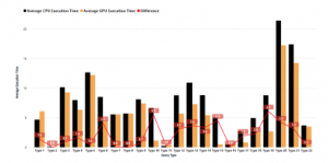
Figure 11: CPU vs GPU Average Run Time

To get closer information, we group the query type 1, 5, 7, 8, 11, 16, 22 and query type 6, 10, 15, 19 and breakdown into the attribute information as shown on Figure 11 There is three information provided by this figure, The black bars, orange bars, and red line. The black bars are representing an average of the attribute value for the query type 1,5,7,8,11,16,22, while the orange bars are representing an average of the attribute value for query type 6,10,15,19. The red line is showing the variance between 2 categorys value.

4.3.1       number of groupby

Based on Figure 12, to get the optimal use of GPU processing speed we need to pay attention of this attribute, this attribute represents the number of group by used on the queries, the numbers on Figure 12 shown that GPU can help on speed up the query processing speed if the query has a lesser amount of group by the operator used.

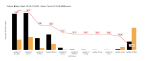
Figure 12: Average Attribute Value by Query Groups

4.3.2       number of column

The number of columns is related to the number of groupby whereas if a query wants to generate an aggregated result within some column information, then group by is mandatory. The difference of this attribute with number of groupby is this attribute also calculate the aggregation used. Based on Figure 13, the numbers proved that GPU co-process is not optimized to deal with a query that has a tremendous amount of column selected.

On Figure 13, the system figured that the more column we try to display on a query, the more ineffective GPU coprocessor works, this confirm if there is a transfer overhead between main memory into GPU memory, as the more columns are trying to be processed the more data also need to be transferred into GPU memory.

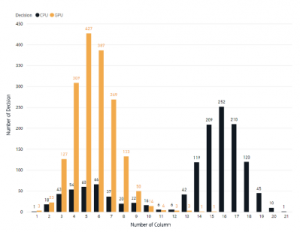
Figure 13: Query Processing Platform Decision Based on Column Count

4.3.3       number of orderby

This attribute is affecting the GPU device processing performance, Figure 12 is showing that a higher amount of order by feature used on the query the more ineffective the GPU becomes. However, these numbers might be affected by the number of columns as in general, order by usually applied to a column.

4.3.4       number of joins

This attribute indicates how many joins used on a query. On Figure 14 we can see, that GPU only optimized if the query join is not more than three tables. The processing speed on GPU starting to increase on five or more join are involved, which makes the system labelled the query to run on CPU only execution.

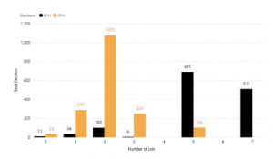
Figure 14: Query Processing Decision Based on Number of Join Used

4.3.5       number of subquery

From the chart, we can see if the current GPU database still not optimized for queries with subquery in it. The query type 1, 5, 7, 8, 11, 16, 22 have a higher amount of subqueries in it, and as the results, the system is determining these types of this query to be run on CPU only mode. Therefore, with this result, we can conclude that if a query has no more than one subquery, it can be run on GPU but, if it has more than 1, the GPU might be not a correct platform to run those queries.

4.3.6       number of wildcard

From the chart, we can conclude that usage of wildcard operators on a query is still not optimized to be run on GPU Co-process database. This result also strengthens by Figure 15. In this figure, we can see that there is the least decision made for a query to run on GPU co-processor if there is a wildcard operator used on those queries.

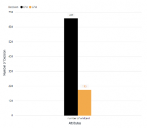
Figure 15: Number of Decision Value Comparison for Query With Wildcard

4.3.7       number of having

The chart showed the query type 1, 5, 7, 8, 11, 16, 22 are having a higher number of having attributes, this meaning there might be not the right choice to run a query with having an operator in it. However, this situation also can be changed if the query has another component that strongly optimized on GPU such as a lower number of columns, joins, or a higher number of aggregations.

4.3.8       number of avg, number of count and number of sum

On Figure 11, we can see that query type 1, 5, 7, 8, 11, 16, 22 have a lower number of sum, but higher number of avg and number of count. However, the number of avg and number of count have a minimal number on it. Hence we reveal the whole number of aggregation, and as we can see on Figure 16, almost all aggregation type query is run faster on GPU, this result confirms the previous research that says the GPU processing is very powerful on an aggregation query type.

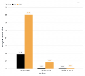
Figure 16: Average Attribute Value for Aggregation

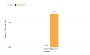
Figure 17: Number of Left Join Value Comparison Between CPU and GPU Decision

4.3.9       number of filter

Based on Figure 11, we can see if the GPU can overrun the CPU processor on query with a high amount of filter used on those queries, this proves the GPU SIMD capabilities, as the filtering can be done simultaneously in a parallel way on GPU devices. With this result, we can conclude that if we wanted to run a query with filters on it, GPU co-process could do faster than the CPU only processing. There is a limitation of the above analysis, query Type 1, 5, 7, 8, 11, 16, 22 and query type 6, 10, 15, 19 are do not cover number of left joins; therefore we will separate the analysis for left join. As shown on Figure 17, there is no decision made on CPU when there is left outer join operation query. However, the dataset we use in this research still does not have many outer join operator, which mean this result might be different on another environment where the outer join operator is very commonly used on the real-life ad-hoc queries.

With this result, an appearance of The GPU database is suitable for a simple query with a fewer number of joins and columns selected.

However, the processing speed comparison is significantly higher for query type, which has aggregation in it and a higher amount of filters.

Table 6 is a summarized table for fundamental understanding for an impact of the use of each query function. The Performance impact have High and medium value; this value is determined by comparing the amount of each feature on both GPU and CPU. If the variance is greater than 50% then the value is high, and vice versa, the value will be medium, and if the variance is lower than 20% then the impact grouped as low. As on this research, there is no variance under 20% there is no Low impact grouped.

Table 6: Query Attribute Impact Summary

Feature	Performance Impact	Suitable Platform*
Number Of Joins	High	GPU
Number Of Left Joins	High	CPU
Number Of Inner Joins	High	CPU
Number Of Filter	Medium	CPU
Number Of Count	High	GPU
Number Of Sum	High	GPU
Number Of Min	High	CPU
Number Of Avg	High	GPU
Number Of Column	High	CPU
Number Of Groupby	High	CPU
Number Of Orderby	High	CPU
Number Of Having	High	GPU
Number Of Wildchar	High	CPU
Number Of Squery	Medium	CPU

* The Suitable Platform is valid when feature value has high amount, when the value is low, the suitable Platform result is the opposite.

5. Conclusions & Future Works

In this paper, we have explored the open issues on the GPU database and introduce a machine learning model to enhance the GPU memory usage on the system by eliminating unnecessary data processing on GPU. As on specific queries, CPU processing also still outperform the GPU processing speed, this model also can prevent the system from choosing the processing platform based on the query type wrongly. On the real-world, this approach can be implemented by embed the proposed framework into the upper system. As the OmniSci is a database component which has data related task such as store the data and process the query then pass the processed data into the upper layer, hence to use this database, the upper layer also needed where all the codes and logic happen. In this interface, we can embed the framework and helps the system to choose the right execution platform.

The proposed approach works by automatically parses the input queries, the parsed query then identified by the system to find the parameters that might affect the GPU processing speed, the system then put the query information into the machine learning, and as a result, the system will determine if those input query will be executed on GPU or CPU. To test both CPU and GPU performance on the same system, we use docker as a CPU processing platform, although, to validate the performance result, we conduct a preliminary study to check if there is any speed difference between docker OmniSci vs Linux OmniSci, and as a result, there is no speed difference between them. The machine learning model was validated using cross-validation function within five-folds, and the best result is the Random Forest algorithm with 95% F1-Score value following by

AdaBoost on 94% and KNN with 93%. However, from the Random

Forest, KNN, and AdaBoost, KNN has the fastest training time, 8.25 times faster than the Random Forest, and 180.5 times faster than Adaboost. Hence with this result, we are choosing KNN as the best algorithm for this framework. From the query side, we also found that usage of filter and subqueries is not affecting the performance difference between CPU only processing vs GPU co-process setup. However, the number of columns on a query is a crucial performance for optimal processing time on a GPU co-processor setup. The more column needs to be shown on a query result, the more challenging for a GPU device to process it. There are some limitations to this research. First, we are using a middle tier of a graphics card to test the model. Hence if the same method tested on a higher-end tier of graphics cards such as tesla cards, the result might differ. Second, due to OmniSci feature limitation, the GPU data transfer time is not measured on this research. This leads to limited analysis results as we can only see the total query processing time of GPU. Third, due to OmniSci limitations, we unable to identify the data type of each selected column on a query. This may lead to reduced model accuracy as processing time required to process textual data, and numerical data may differ. Forth, the data used for this research is not a real user ad-hoc queries, which mean the query used in this research may not cover all the query scenario used by real users.s

As for the future works, this method needs to be tested on a higherend tier of graphics cards to see if there are still limitations that happened on higher-end tier graphics cards. Second, to get a better insight to do a more detailed analysis, the GPU data transfer time needs to be measured, by measuring the transfer time we can see if the I/O bottleneck happens or not. Third, the query parser may need to be adjusted to calculate the number of numerical columns and non-numerical column selected. This may increase the accuracy of the model. Moreover, this algorithm should be applied to the real-world data and ad-hoc user query where all query types, functions all used on it. The researcher is also planning to extend the work by enhancing the current machine learning model into an unsupervised learning method, where the system will have an ability to learn by itself based on inputted user’s query, hence the longer the system work, the smarter it becomes. Unsupervised learning also can reduce the time for initial training in the model.

Conflict of Interest

The authors declare no conflict of interest.

Acknowledgment

We thank Tjeng Wawan Cenggoro from NVIDIA AI R&D Center Bina Nusantara University for helpful feedback and discussions.

1.  KK Yong, Hong Ong, and Vooi Yap. Gpu sql query accelerator. International Journal of Information Technology, 22:22, 12 2016.
2.  Sebastian Bre, Max Heimel, Norbert Siegmund, Ladjel Bellatreche, and Gunter Saake. GPU-Accelerated Database Systems: Survey and Open Challenges. In Abdelkader Hameurlain, Josef Kng, Roland Wagner, Barbara Catania, Gio- vanna Guerrini, Themis Palpanas, Jaroslav Pokorn, and Athena Vakali, editors, Transactions on Large-Scale Data- and Knowledge-Centered Systems XV, vol- ume 8920, pages 1–35. Springer Berlin Heidelberg, Berlin, Heidelberg, 2014. ISBN 978-3-662-45760-3 978-3-662-45761-0.
3. Andreas Meister, Sebastian Breß, and Gunter Saake. Toward gpu-accelerated database optimization. Datenbank-Spektrum, 15(2):131–140, Jul 2015.
4. Peter Bakkum and Kevin Skadron. Accelerating SQL Database Operations on a GPU with CUDA: Extended Results. page 21.
5.  Iya Arefyeva, David Broneske, Gabriel Campero, Marcus Pinnecke, and Gunter Saake. Memory management strategies in cpu/gpu database systems: A survey. In Stanisaw Kozielski, Dariusz Mrozek, Pawe Kasprowski, Bozena Maysiak- Mrozek, and Daniel Kostrzewa, editors, Beyond Databases, Architectures and Structures. Facing the Challenges of Data Proliferation and Growing Vari- ety, pages 128–142, Cham, 2018. Springer International Publishing. ISBN 978-3-319-99987-6.
6. Esraa Shehab, Alsayed Algergawy, and Amany Sarhan. Accelerating relational database operations using both CPU and GPU co-processor. Computers & Electrical Engineering, 57:69–80, January 2017.
7. Jayshree Ghorpade. Gpgpu processing in cuda architecture. Advanced Com- puting: An International Journal, 3:105–120, 01 2012.
8. Jun Sui, Chang Xu, S.C. Cheung, Wang Xi, Yanyan Jiang, Chun Cao, Xiaoxing Ma, and Jian Lu. Hybrid CPUGPU constraint checking: Towards efficient context consistency. Information and Software Technology, 74:230–242, June 2016.
9. David B. Kirk and Wen mei W. Hwu. Programming Massively Parallel Pro- cessors: A Hands-on Approach. Morgan Kaufmann, 2012. ISBN 0124159923.
10. Chris Gregg and Kim Hazelwood. Where is the data? Why you cannot debate CPU vs. GPU performance without the answer. In (IEEE ISPASS) IEEE IN- TERNATIONAL SYMPOSIUM ON PERFORMANCE ANALYSIS OF SYSTEMS AND SOFTWARE, pages 134–144, Austin, TX, USA, April 2011. IEEE. ISBN 978-1-61284-367-4.
11.  OmniSci Technical White Paper.
12.  Fabian Pedregosa, Gae¨l Varoquaux, Alexandre Gramfort, Vincent Michel, Bertrand Thirion, Olivier Grisel, Mathieu Blondel, Peter Prettenhofer, Ron Weiss, Vincent Dubourg, et al. Scikit-learn: Machine learning in python. Journal of machine learning research, 12(Oct):2825–2830, 2011.
13. Leo Breiman. Random forests. Machine learning, 45(1):5–32, 2001.
14.  Abraham J Wyner, Matthew Olson, Justin Bleich, and David Mease. Explain- ing the success of adaboost and random forests as interpolating classifiers. The Journal of Machine Learning Research, 18(1):1558–1590, 2017.
15.  Vivek Narayanan, Ishan Arora, and Arjun Bhatia. Fast and Accurate Sentiment Classification Using an Enhanced Naive Bayes Model. In Hujun Yin, Ke Tang, Yang Gao, Frank Klawonn, Minho Lee, Thomas Weise, Bin Li, and Xin Yao, editors, Intelligent Data Engineering and Automated Learning IDEAL 2013, pages 194–201. Springer Berlin Heidelberg, 2013. ISBN 978-3-642-41278-3.
16.  Paraskevas Tsangaratos and Ioanna Ilia. Comparison of a logistic regression and na¨ive bayes classifier in landslide susceptibility assessments: The influence of models complexity and training dataset size. Catena, 145:164–179, 2016.
17.  David W Hosmer Jr, Stanley Lemeshow, and Rodney X Sturdivant. Applied logistic regression, volume 398. John Wiley & Sons, 2013.
18.  Jesus Maillo, Sergio Ram´irez, Isaac Triguero, and Francisco Herrera. knn-is: An iterative spark-based design of the k-nearest neighbors classifier for big data. Knowledge-Based Systems, 117:3–15, 2017.
19.  Yoav Freund, Robert Schapire, and Naoki Abe. A short introduction to boost- ing. Journal-Japanese Society For Artificial Intelligence, 14(771-780):1612, 1999.
20.  TPC BenchmarkTM H Standard Specification Revision 2.18.0.
21.  Naga K. Govindaraju and Dinesh Manocha. Efficient relational database man- agement using graphics processors. In Proceedings of the 1st international workshop on Data management on new hardware – DAMON ’05, page 1, Baltimore, Maryland, 2005. ACM Press.
22. Kevin Angstadt and Ed Harcourt. A virtual machine model for accelerating relational database joins using a general purpose gpu. In Proceedings of the Symposium on High Performance Computing, HPC ’15, pages 127–134, San Diego, CA, USA, 2015. Society for Computer Simulation International. ISBN 978-1-5108-0101-1.
23. Yue-Shan Chang, Ruey-Kai Sheu, Shyan-Ming Yuan, and Jyn-Jie Hsu. Scaling database performance on GPUs. Information Systems Frontiers, 14(4):909–924, September 2012.

(Click Here)

(Click Here)