1. Introduction

Thin shell (TS) electromagnetic models have been presented by many author [1]-[3] to neglect meshing volumic shells (Fig. 1, left) and are introduced by surfaces (Fig. 1, right) with interface conditions (ICs) related to 1-D analytical distributions across the shell thickness.

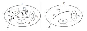
Figure 1: Volumic shell Ω_t (left) and IC Γ_t (right).

In general, the ICs cancel corner and curvature effects, and lead to inaccuracies of magnetic fields, eddy current losses and Joule power losses in the neighbouring regions of geometrical discontinuities around borders and corners, changing with the thickness. So as to overcome with this disadvantage, a subproblem method (SPM) with a magnetic vector potential formulation for improving errors next to corners and curvatures occurring from the TS has recently presented by many author [4, 5].

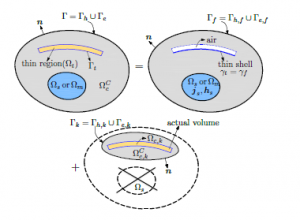
Figure 2: Decomposition of full problem into several SPs.

The idea of this article is to present an extension of the oneprocess SPM that proposes the magnetic field formulation. The hearth of this technique is based on a SPM, which consists in splitting a complete/full problem (including of stranded inductors and magnetic or conductive thin structures) into two subproblems (SPs), the complete/full solution being the superposition of all solutions for each SPs.

A problem involving stranded inductors and TS models (Fig. 2, top right) is first considered on a simplified mesh. The obtained solution is then adjusted by a improvement problem with the actual volume thin regions (Fig. 2, bottom). In this process, each SP is constrained by volume sources (VSs) or surface sources (SSs), where VSs present variations of the permeability and conductivity in volume thin regions and SSs express variations of ICs across surfaces from previous SPs. Each process allows to inherit the previous sources/solutions for new SPs instead of starting a new

complete problem for each new geometries as a traditional finite element method (FEM) [6].

2. Sequence of Pertubation Technique

2.1        Magnetodynamic subproblem

In the heart SPM, a canonical magnetodynamic SP p considered at step p is solved in a domain Ω_p, with boundary ∂Ω_p = Γ_p = Γ_h,p ∪ Γ_e,p. The eddy current density is defined in conducting part

where h_p is the magnetic field (A/m), b_p is the magnetic flux density (T), e_p is the electric field (V/m), ^j_s,p is the electric current density

(A/m²), µ_p is the magnetic permeability (H/m), σ_p is the electric conductivity (S/m) and n is the unit normal exterior to Ω_p. The source fields (b_s,p and e_s,p) in (2a-b) are VSs, and the source fields (j_su,p and k_su,p) in (3a-b) are SSs. In general, SSs are defined as zero for classical homogeneous BCs. ICs can express their discontinuities across the negative and positive sides (γ⁺_p and γ⁻_p) of any interface γ_p (with the notation [·]_γp = |_γ+_p − |_γ−_p ) in Ω_p. For the idealized thin regions, these ICs are SSs that have to account for special phenomena ocurring between two sides of γ_p [4, 5].

2.2        Relations of SPs with SSs and VSs

As proposed in [3], the relation between SPs p (TS models and volume corrections) are respectively defined via SSs and VSs. A volume thin region Ω_t,p in Ω_c,p is initially removed from Ω_i and then defined with the double layer TS surface Γ_t,p. For the magnetic field formulation (h_p-conformal formulation), the coefficient discontinuity h_d,t,p of the tangential component h_t,p = (n × h_p) × n of h_p is presented across via the TS model, i.e. [3]

where the discontinuous component (h_d,t,p) of the field h_t,p is considered as zero along the TS border, which neglects the present magnetic fields. To present this discontinuity, it gets [3]

where h_c,p is the continuous component of h_p. The expressions (5) also applies on Γ_t,p for the tangential components h_t,p, h_c,t,p and hd,t,p.

The TS model combined with the ICs and BCs of the impedance BC type [3] are presented through h_c,t,p and h_d,t,p, that is

where d_p is the local thickness of the TS, δ_p is the skin depth, ω = 2πf with f is the frequency, j is the imaginary unit and ∂_t ≡ jω. It should be noted that the term −n × e_i|_Γ−_t,i in (7) is presented as a SS for the SPs.

As presented, the inaccuracy on the TS solution of a problem p (e.g, p = u) is then improved by a volume correction SP k (e.g., p = k) which scopes with the TS hypothesis [3]. The changes from a TS region (µ_u and σ_u for SP u) to a volume thin region (µ_k and σ_k for SP k), the field sources (h_s,k and ^j_s,k) in (2a-b) are defined for the total fields [5, 8]

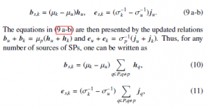
where q ∈ P (total SPs) except the current SP u relates to the sources (b_s,k and e_s,k) via their last calculated corrections of h_q and j_q.

3. Finite element weak formulation

3.1        h_p-magnetic field formulation with source and reaction fields

The weak magnetic field formulation (h_p-conformal formulation) is obtained via the Faraday’s law (1c) [5, 8, 9]. The magnetic field h_p is decomposed into two parts, h_p = h_s,p + h_r,p, where h_s,p is the source magnetic field presented via curl h_s,p = j_s,p, and h_r,p is the reaction magnetic field. In Ω^C_c,p, the field h_r,p is expressed through a scalar potential φ_p, i.e. h_r,p = −gradφ_p. The weak forms for SPs p (p = u, k…) are [10]

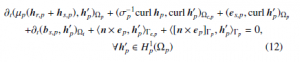
where H¹_p(Ω_p) including the basis functions for h_p as well as for the test function h⁰_i is a curl-conform function space presented in Ω_p. Notation of (· , ·)_Ωi is volume integral in Ω_p and < · , · >_Γp is the surface integral on Γ_p of the product of their vector field arguments. The term on surface integral Γ_e,p gives as a natural BC of type (3 b), usually zero. It should be noted that the source field h_s,p in (12) is performed through a projection technique [11] of a known distribution j_s,u, i.e.

3.2        Weak formulation for the TS model

The TS model [3] occurred in the general equation (12) is defined a free discontinuous h_d,t,u (p =u) along the TS and h_d,u in the exterior region related to Γ⁺_u and a BC n × e_u|_Γu+. This discontinuity is used as a test function h⁰_u (h⁰_u = h⁰_c,u + h⁰_d,u) in (12), where term contributions in the volume integrals in Ω_u are defined on the positive side of the TS. For that, the term h[n × e_u]_Γu , h⁰_ui_Γu is analysed as h[n × eu]Γu , h0uiΓu = h[n × eu]Γu , h0c,uiΓu + hn × eu|Γu+, h0d,uiΓu+

where with h⁰_d,u is equal to zero on the negative side of TS Γ_u−

[11]. Moreover, the term h[n × e_u]_Γu , h_c⁰i_Γu and hn × e_u|_Γu+, h_d⁰ i_Γu+ are presented by (6) and (7), respectively. Therefore, (3.2) becomes

where the surface integral term on Γ_e,u − Γ_t,u is usually considered as zero on a natural BC.

3.3        Projection of solutions between sub-models

In the strategy SP technique, the solutions found from a previous problem SP u are considered as sources (SSs and VSs) in a subdomain Ω_s,k ⊂ Ω_k of the SP k (current SP), e.g. from SP u to SP k. At the discrete level, the field h_u in the mesh of the SP u is transferred to the mesh ot the SP k (i.e. h_u,k−proj). This will be performed via a projection technique [11] of its curl limited to Ω_s,k.

The field h_u,_k−proj is defined

where H_k¹(Ω_s,k) is a curl-conform function space containing the projection of h_u and the test function h⁰ in the mesh k. Directly projecting h_u instead of its curl will give numerical errors as estimating its curl.

3.4        Improvement of the TS model

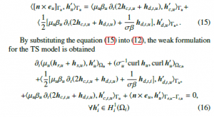
The inaccuracies of the TS solution obtained in SP u is now improved by the actual volume SP k via VSs defined in (10) and (11). They are taken into account the changes from µ_u and σ_u in the TS model to µ_k and σ_k in the volume shell. These VSs also appear in (12) via the volume integrals (∂_t(b_s,k, h⁰_k)_Ωk and (e_s,k,curl h⁰_k)_Ωk ). The weak form for SP k is written as

where the field e_u is also performed via an electric problem [9]. As a sequence, the field h_u is transferred to the mesh of SP k via (17), where Ω_s,u is limited to a single layer surrounding of the volumic shell. In the same time to the VSs in (12), SSs related to ICs [3], [5] have to extract the TS discontinuities, i.e, h_d,k =−h_d,u and [n × e_k]_Γts,k = −[n × e_u]_Γts,u . The involved trace [n × e_u]_Γts,k is generally defined through other integrals in (12), with Γ_ts,u = Γ_ts,k,

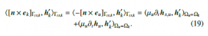
The surface integral in (19) is implemented in the step u. At the discrete level, the limitation of the two volume integrals in (19) is defined in a single layer of FEs on both sides of Γ_t,u touching γ_k⁺ = ^γ_u⁺ = Γ⁺_t , because it involves only the trace n × h⁰_k|_γk+.

4. Numerical test

The practical test is a TEAM workshop problem (problem 21, model B) [12] including two coils and a magnetic shielding plate (Fig. 3). The test problem is considered in both 2-D and 3-D models.

Figure 3: Geometry of the test problem 21 (model B).

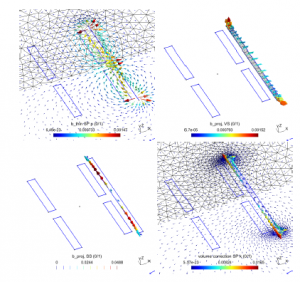
Figure 4: Magnetic flux densities for the TS solution SP u (b_u, top left) and volume correction solution SP k (b_k, bottom right). Projections of SP u solutions (b_proj, VS, top right) and (b_proj, SS, bottom left) in the SP k.

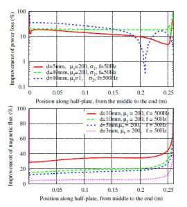
Figure 5: Relative improvements of the joule power loss density (top) and the magnetic flux (bottom) along the thin plate, with σ_plate =6.484 MS/m.

The first case is tested with a 2-D model: The SP u with the inductors and TS FE magnetodynamic model is solved on a lighter mesh (Fig. 4 (b_u), top left). A volume correction SP k then replaces the TS FEs with the classical volume FEs containing an actual region of the thin plate and its surrounding, with a suitable refined mesh without including the inductors anymore (Fig. 4 (b_k), bottom right). The projections of TS solution in TS SP u for the VS and SS are respectively pointed out (Fig. 4 (b_proj, VS), top right) and

(Fig. 4 (b_proj, SS), bottom left). The relative improvements of the joule power loss density and the magnetic flux along the plate are depicted in Fig. 5. They can touch several tens of percents near the end of the TS, such as 80% (Fig. 5, top) and 85% (Fig. 5, bottom), with d = 10 mm and δ = 1.977 mm for both cases. For d = 10 mm, the inaccuracy is lower than 50% (Fig. 5, top) and 55% (Fig. 5, bottom).

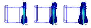
Figure 6: Colored maps of eddy current densities indicating the regions with relative volume improvements greater than 2% for d = 5 mm, 7.5 mm and 10 mm (from left to right), f = 50 Hz, µ_plate = 200 and σ_plate =6.484 MS/m.

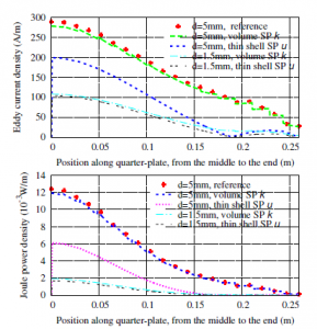
Figure 7: Eddy current density (top) and joule power loss density (bottom) for the TS and the volume corection along the vertical half edge (z-direction) (f = 50 Hz, µ_plate = 200 and σ_plate =6.484 MS/m).

The next test is considered with a 3-D model: The errors of the TS model SP u are shown in Fig. 6 (from left to right). They increase with plate thickness, specially near the ends of the plate, are perfectly improved whatever their order of magnitude. The accuracy of the improvement is directly related to the volume correction of the plate and its surrounding.

The inaccuracies on the eddy current density and joule power loss density of TS model (SP u) are improved by the significant volume correction (SP k) (Fig. 7. The inaccuracies on the local fields (eddy current density and joule power loss density) along the vertical half edge (z-direction) near the plate ends reaches 60% (Fig. 7, top) and 80% (Fig. 7, bottom), respectively, with δ = 2.1mm and d = 5mm. The volume corrections are then compared to be similar the reference solutions (obtained from the FEM) for different parameters in both cases.

5. Conclusions

In this study, a perturbation Finite Element Approach has been proposed with a magnetic field formulation for a one-way coupling in order to improve the errors around edges and corners inherent to the TS FE assumptions. The correctly improving on the local fields of magnetic flux densities, eddy current losses and joule power losses is successfully achieved surrounding the borders and corners of the TS structures. The proposed method has been developed for the one-way coupling in two steps. All the processes of the method have been successfully validated on the international practical problem (TEAM workshop problem 21, model B) [12].

The source-codes of the this technique have been being extended based on the source-codes of the SPM that was developing by author and two Prof. Patrick Dular and Prof. Christophe Geuzaine at the Dept of Electrical Engineering and Computer Science, University of Liege, Belgium. They will be then ran and simulated in the background of the Getdp (http://getdp.info) and Gmsh (http://gmsh.info) softwares developed by Prof. Patrick Dular and Prof. Christophe Geuzaine [13, 14]. These are the open-source codes for anyone to be able to write adapt source-codes for solving studied problems (if possible).

1. L. Kra¨henbu¨hl and D. Muller, “Thin layers in electrical engineering. Examples of shell models in analyzing eddy- currents by boundary and finite element methods,” IEEE Trans. Magn., vol. 29, no. 2, pp. 1450–1455, 1993.
2.  Tsuboi, H., Asahara, T., Kobaysashi, F. and Misaki, T. (1997), “Eddy current analysis on thin conducting plate by an integral equation method using edge elements,” IEEE Trans. Magn., Vol. 33, No. 2, pp. 1346-9.
3. C. Geuzaine, P. Dular, and W. Legros, “Dual formulations for the modeling of thin electromagnetic shells using edge elements,” IEEE Trans. Magn., vol. 36, no. 4, pp. 799–802, 2000.
4. P. Dular, Vuong Q. Dang, R. V. Sabariego, L. Kra¨henbu¨ hl and C. Geuzaine, “Correction of Thin Shell Finite Element Magnetic Models via a Subproblem Method,” IEEE Trans. Magn., vol. 47, no. 5, pp. 1158–1161, 2011.
5. Vuong Q. Dang, P. Dular, R. V. Sabariego, L. Kra¨henbu¨ hl and C. Geuzaine, “Subproblem Approach for Thin Shell Dual Finite Element Formulations,” IEEE Trans. Magn., vol. 48, no. 2, pp. 407–410, 2012.
6. S. Koruglu, P. Sergeant, R.V. Sabarieqo, Vuong. Q. Dang and M. De Wulf “Influence of contact resistance on shielding efficiency of shielding gutters for high-voltage cables,” IET Electric Power Applications., Vol. 5, No. 9, pp.715-720, 2011.
7. Vuong Quoc Dang and Quang Nguyen Duc, “Coupling of Local and Global Quantities by A Subproblem Finite Element Method Application to Thin Re- gion Models,” ASTESJ, vol. 4, no. 2, pp. 40–44, 2019.
8. Vuong Quoc Dang and Quang Christophe Geuzaine, “Using edge elements for modeling of 3-D Magnetodynamic Problem via a Subproblem Method,” Sci. Tech. Dev. J.; 23 (1), pp. 439–445, 2020.
9. P. Dular and R. V. Sabariego, “A perturbation method for computing field distortions due to conductive regions with h-conform magnetodynamic finite element formulations,” IEEE Trans. Magn., vol. 43, no. 4, pp. 1293-1296, 2007.
10.  Vuong Q. Dang, P. Dular, R. V. Sabariego, L. Kra¨henbu¨hl, C. Geuzaine “Sub- problem Approach for Modelding Multiply Connected Thin Regions with an h-Conformal Magnetodynamic Finite Element Formulation,” in EPJ AP., vol. 63, no. 1, 2013.
11.  C. Geuzaine, B. Meys, F. Henrotte, P. Dular and W. Legros, “A Galerkin projection method for mixed finite elements,” IEEE Trans. Magn., Vol. 35, No. 3, pp. 1438-1441, 1999.
12.  Zhiguang CHENG1, Norio TAKAHASHI2, and Behzad FORGHANI, “TEAM Problem 21 Family (V.2009),” Approved by the International Compumag Soci- ety Board at Compumag-2009, Florianopolis, Brazil.
13.  C. Geuzaine and J.-F. Remacle “Gmsh: a three-dimensional finite element mesh generator with built-in pre- and post-processing facilities,” International Journal for Numerical Methods in Engineering 79(11), pp. 1309-1331, 2009.
14.  P. Dular and C. Geuzaine “GetDP reference manual: the documentation for GetDP, a general environment for the treatment of discrete problems,” University of Liege, 2013.

(Click Here)

(Click Here)