1. Introduction

This work is an extension of conference paper “Optimization of the Program for Run Time Parametrical Identification for ARM Cortex Processors” originally presented in “2018 International Conference on Industrial Engineering, Applications and Manufacturing (ICIEAM)” [1]. Conference paper has the results obtained only with the 32-bit armv7 processor. The results obtained with the 64-bit armv8 processor are added in the current paper. Also, the questions of alignment data in memory and leftovers processing during vectorization are considered.

Nowadays most of the micro-controllers are based on inexpensive but at the same time powerful ARM processors. High computing abilities of these processors allow to realize not only simple PID-controllers but more sophisticated adaptive controllers. Adaptive digital controllers are indispensable for technological processes which require high quality of control. In this case oscillation and overshooting are inadmissible and setting time must be minimal. And digital controllers are able to improve process control performance significantly. The theory of digital control systems was developed in 70-80 years of the last century. In particular, K. Astrom and B. Wittenmark [2] and R. Iserman [3] showed that digital controllers are the best when aperiodic transient processes are wanted and described how to make state variable modal digital controller capable to provide any in advance known characteristics of the transient process. When an object of control is timeinvariant it is possible to use experimental data and find out the coefficients of the digital transfer function of this object and the coefficients of digital modal controller and digital observer preliminarily. These calculations are carried out only once and their results may be used as the constants in the program for direct digital control. But when the object of control is unstable i.e. its characteristics drift with the time, or its characteristics are non-linear and its linear approximation depends on operating point, all above mentioned calculations must be made repeatedly at run time within controller itself with the pace of technological process. And in this case time consumption for such calculations may be crucial. In other case quality of control may decrease drastically.

2. Using least squares method for parameter evaluation

The most substantial part of calculations in discussion is the object’s parameter estimation, i.e. the process of finding out its digital transfer function coefficients. And the task of this article is to show how time consumption of the program for parameter estimation may be reduced. The novelty of this work is in making new program realization of the least-squares method that includes refusing of function decomposition of the code. As a result, some intermediate matrices may be dropped and outer loops of sequential stages of calculations may be linked. Such a decision allows reducing the program’s time and memory consumption that is very significant in the case of real-time applications based on the microcontrollers. Also, for further optimization, the code parallelism and different ways of data parallelism are added to the program and a comparison of the obtained results is made.

The general method of the object of control parameter estimation is the least-squares method or LSQ [4]. Using LSQ, one can get a transient function of the object in a discrete form. The coefficients of this transfer function are used to find out parameters for tuning adaptive dynamic regulators [3].

Despite the fact that LSQ is a rather old method, there are still a lot of publications connected with it. Each of them is devoted to special ussue. For example, identification of nonlinear systems [5], time-varing magnetic field analysis [6], signal processing [7], lines approximation in multidimentional space [8]. But among them, researches connected with LSQ utilization at microcontrollers when amount of RAM is limited and time constraint are strict are not found.

LSQ is widely used in many fields of applied calculations and it’s realization is available in many program libraries. First of all must be mentioned lapack library (https://www.netlib.org/lapack/) – standard library that may be found in many Unix-like operating systems. Another widely used library is gnu scientific library or gsl (https://www.gnu.org/software/gsl/). These libraries use QR-decomposition [9] for solving LSQ problem. This method is considered to be one of the fastest for the big dimension tasks.

But the objects of control usually are described with the models that have order between 2 and 6. So it is reasonable to suggest that program based on QR-decomposition will spend more time making preliminary computing than useful one when applied to such small systems. And with the micro-controllers situation when it will be not enough memory for such libraries is also possible.

To check this hypothesis the program was written that applied matrix operations as LSQ suggests [9] and as is shown in (1):

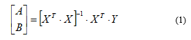
where X – matrix with the dimension of Nx2M filled with values taken from input and output of the object with the regular intervals of time; Y – vector with the dimension of N filled with the values taken from the output of the object; A – output vector with the dimension of M having coefficients of transfer function denominator; B – output vector with the dimension of M having coefficients of transfer function nominator; L – number of experimental points; M – order of the object of control; N = L – M – number of equations.

Covariance matrix is represented in (2):

Equation (2) that is the part of (1) plays special role and is used for evaluation of parameters dispersion [10].

How to fill matrix X and vector Y with the experimental values is shown in [3].

Other reasons to write such program are the following:

At the first, for correct parameter estimation of the object of control the trace of covariance matrix must be minimal and the value of this trace depends mainly on sampling period [11]. This means that at the first stage of parameter estimation time step may vary and alongside with the model’s parameters the trace of covariance matrix must be computed. Getting the covariance matrix is the part of LSQ method, so it’s trace may be computed when direct matrix operations are involved. While using library functions this data are hidden inside them. And to get covariance matrix one needs to repeat a bigger half of computations already made.

At the second, during LSQ parameter evaluation some dynamically allocated matrices are used for storing intermediate data. Each time when library function is called the memory is allocated for them and then released. While using our own code we can allocate memory for intermediate matrices only once and then use them with every next time step.

As equation (1) shows LSQ consists of matrices multiplication and matrix inversion. Matrices multiplication may be written from scratch. An example of matrix inversion can be found in the Internet (http://www.programming-techniques.com/2011/09/numerical-methods-inverse-of-nxn-matrix.html). This program realizes the Gauss-Jordan method [12].

3. Program Testing and Optimization

3.1.  General Information about Testing

For realization and testing of the programs singleboard mini-computers CubieBoard-3 and Odroid-C2 were used. CubieBoard-3 has two core CPU CORTEX-A7 (ARMv7) with the frequency 1GHz and 2G of RAM. Operating system Linux Ubuntu 18.04.1 with the kernel 4.19.57 is installed on this computer alongside with gcc compiler v 7.4.0. Odroid-C2 has quad core CPU CORTEX-A53(ARMv8) with the frequency 1.5GHz and 2G of RAM, operating system Linux Ubuntu 16.04.09 with the kernel 3.14.79 and gcc compiler 5.4.0. For the conference paper [1] programs were made with the gcc v 4.6.3, so results presented in this article may slightly differ, first of all due to the fact that the realization of optimization in these compilers is not identical.

For program realization, the C++ language was chosen. It’s a common practice nowadays even for embedded systems. If you do not use classes with the virtual functions, the productivity of the result code is almost the same, and at the same time, the full power of C++ as a language of generic programming is available.

All programs were compiled with the -O2 level of optimization.

Working with the matrices, one must decide how to store them in memory. First way suggests using dynamic one dimensional flat vectors. Matrix elements in this case are accessible with the function or overloaded operator () taking as arguments row and column number. E.g. getElem(X,i,j) or X(i,j). Second way suggests using dynamic two dimensional arrays. In this case X[i] is a vector of pointers containing the addresses of matrix’s rows and X[i][j] is an element of matrix. First way is considered to be slightly faster as the data occupy continues space in memory. But for an adaptive controller second way is more suitable, because in this case matrix X must be renewed with every next step in time. Old data must be removed and new once added. With the flat vector all elements counted with thousands will be moved within this vector from the end to the beginning. But with the two-dimensional array only pointers counted with tens will be moved.

3.2.  Comparison of Code Using Library Functions and Code Using Direct Operstion with the Matrices

To compare time consumption for LSQ 3 programs were written. The first used function dgel from the lapack library, the second used function gsl_linalg_QR_lssolve from the gnu scientific library and the third realized equation (1) using self-written functions for matrix multiplication and inversion. Time consumption for the calculations was found out as the difference between the time measured before and after the calculations. To measure time the function clock_gettime was used.

Time consumption were determined with the matrices of the following dimensions MxN: 2×40, 3×60, 4×80, 5×100, 6×120, 7×140, 8×160 and 10×200. Objects of higher orders require more experimental points. But this does not mean that to evaluate parameters of the for example 4 order object, one must use exactly 80 experimental points. It is just an average value.

The matrix X and vector Y were filled with the random numbers because we need to get not the results of LSQ-evaluation but only time consumption for getting them.

Calculations for each program and for each dimension were repeated 5 times. Maximum and minimum were removed and out of the rest three measures, an average value was calculated. To run programs, calculate time consumption and to make plots the special script in Python language was written. The resulting plots with the time consumption against object order are shown in Figure 1 for CubieBoard3 and Figure 2 for Odroid-C2.

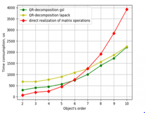
Figure 1: Time consumption for LSQ parameter estimation against object’s order by the programs with the double precision numbers on CubieBoard-3.

The plots in Figures 1 and 2 show that the program that uses matrix operations takes less time then library functions for the tasks of small dimensions. But this program must be rearranged in order further to improve its efficiency.

First, decision must be made is there any sense to replace the double precision variables with the single precision variables or with the fixed-point ones.

3.3.  Time consumption for Carring out Arithmetic Operations

For this purpose, it will be useful to find out how many time take arithmetic operations with the operands of the different types. And proper program with the three operands expression was written and run on CubieBoard-3 and Odroid-C2 computers:

a = b # c

where # in turn is + – * and /; b=2; c=3.

The results are shown in Table 1.

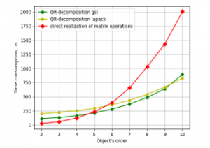
Figure: 2. Time consumption for LSQ parameter estimation against object’s order by the programs with the double precision numbers on Odroid-C2.

Table 1: Time Consumption in μs for Carrying out 1000 Operations on Single-Board Computers CubieBoard 3 and Odroid-C2

Variable type	Operation
	Addition	Subtraction	Multiplication	Division
CubieBoard-3
int	13,5	13,5	14,6	30,2
long	13,5	13,5	14,6	30,3
float	14,6	14,6	14,6	29,2
double	14,6	14,6	17,7	43,8
Odroid-C2
int	7,1	7,1	8,5	8,5
long	7,1	7,1	9,1	8,5
float	9,8	9,8	9,8	15,6
double	9,8	9,8	9,8	21,5

As Table 1 shows, the time consumption for processing integer variables is less than the time for processing floating point variables by 8% for armv7 and 28% for amrv8. But realization of LSQ in adaptive controller requires support of numbers in wide range of values. For example, parameter evaluation of the 3 order object using the experimental results where input varies between 0.0 and 1.0 and output between 0.0 and 200.0 will give values in the intermediate matrices varying from 1.0e-3 to 1.0e6. Obviously, integer values can’t be used for such computing.

Time consumption for single precision and double precision floating point variables is identical for addition, subtraction and multiplication at both platforms. But division takes considerably more time especially for double precision variables.

3.4.  Using Single Precision Variables and Parallelism of Code

Time consumption of the program depends not only on time required for the computing but also on cache misses [13]. Float variable takes 4 bytes and double takes 8 bytes. That means that the processor’s cache can hold more data in case of float variables and so, cache misses will be met less often.

There is one more reason to use variables of single-precision:

• The vector unit of ARM-CORTEX-A (ARMv7) processes only single-precision floating-point numbers, and vectorization is a significant source of increasing program efficiency.
• Microcontrollers STM32 has hardware support only for single precision, and software emulation of double precision is rather slow.

Usually, it’s recommended to avoid single precision variables in calculations [14]. But in our case, the dimension of the task is not big. And if to use in the experiments optimal sampling period, well-conditioned matrices will be obtained [11]. LSQ identification of the same object made with double precision and single precision numbers is almost identical. For these calculations, real experimental results obtained with the object with orders 3 and 4 were used.

There is also one more source of program efficiency improving. It is parallelism of code. And gcc compiler supports OpenMP specification, which provides parallelism or multi-threading. The results obtained are presented in Figures 3 and 4.

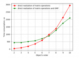
Figure 3. Time consumption for LSQ parameter estimation against object’s order by the programs with the single precision numbers on CubieBoard-3.

The CubieBoard3 computer has 2 core processor and Odroid-C2 has 4 core processor.

Figures 3 and 4 show that using single precision variables instead of double has given about 25% increase in productivity. At the other hand on CubieBoard-3 parallelism has given expected results. I.e. while working with the small matrices synchronization between threads takes more time then parallelism saves it. And for objects with order 7 and higher parallel program becomes faster. But the results obtained on Odroid-C2 show that parallelism instead of increasing productivity reduces it in the whole range. The explanation of this fact may be following. The program calls several functions, and directives for parallel code are placed within them. So OMP preprocessor generates code that creates and cancels threads within each function. At CubieBoard-3 more modern gcc compiler was used with this problem fixed.

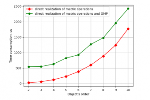
Figure 4. Time consumption for LSQ parameter estimation against object’s order by the programs with the single precision numbers on Odroid-C2.

3.5.  Refactoring of the Code

Next stage of optimization is concerned the code itself.

The first stage is also connected with the problem of cache-missing. In the programs written in C, matrices are allocated in memory row-wise. During multiplication one of the matrices is scanned row by row, and a big piece of data is loaded into cache. But another matrix is scanned column by column, and getting the next element may come to a cache-miss. If preliminary to transpose another matrix it will be also scanned row by row [13].

There is a division in the inner loops of the function that makes matrix inversion. If to calculate the inverse number in the outer loop and replace division with the multiplication we can get another source of the productivity raising.

From the point of view of the structural programming the code must be divided into functions each of them makes logically complete operation. In our case these are matrix multiplication and inversion. But its also known that such structural decomposition may reduce productivity of the program.

If to make one function that makes all calculations in one step it will be possible to take into account specific properties of computing. Informational matrix X^T·X is symmetric and it’s possible to calculate only half of it. And also, it’s possible to get away two intermediate matrices with the sizes [2*M][2*M]. And intermediate matrix [2*M][N] may be replaced with a vector with the size [N]. As a result, the number of cache-misses and total consumption of memory will be reduced. The last is especially significant for STM32 microcontrollers with limited RAM. In this one function, it’s also possible to improve an algorithm. In this new program, the next stage of calculation will be started within an outer loop of the previous stage.

Alongside with the algorithm improvement, OMP directives were added to the code in order to apply parallelism. The resulting program was compiled twice. First time with an OMP flag to get parallel code. And second time without this flag to get code without multithreading.

Calculations were repeated with the same data. The results are presented in Figures 5 and 6.

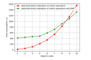
Figure 5: Time consumption for LSQ parameter estimation against object’s order by the programs with the optimized function on CubieBoard-3.

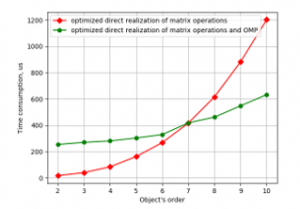
Figure 6: Time consumption for LSQ parameter estimation against object’s order by the programs

Plots in Figures 5 and 6 show that optimization of code gave increasing in speed about 80% for CubieBoard-3 and 50% for Odroid-C2. And using parallelism in one function has given results on Odroid-C2. But also as one can see parallel code is faster only with 7 and higher-order object models. For the object’s model with the order from 2 to 6 nonparallel code is faster and it may be recommended for practical utilization.

And more significant is the fact that the optimized program is faster than programs using lapack and gsl libraries in the whole range from 2 to 10 at both mini-computers.

3.6.  Using Vector Operations

Vectorization is another way to increase program efficiency. ARM-CORTEX-A processors have the vector unit named NEON. This unit has 128-bit registers that enough to keep 4 floating-point numbers. The vector instructions process all numbers in the vectors at one time. Theoretically, it can increase efficiency by 4 times. But usually, this value is less because switching processor’s pipeline between vector and regular registers takes a lot of time. (https://developer.arm.com/products/processors/cortex-m/).

There are many options to use vectorization: special libraries, auto-vectorization of compiler, OMP directives, NEON intrinsics, and assembly code. In our case, the best decision is to use intrinsics. They provide access to all vector instructions and allows them to apply total control of instruction flow comparing with the auto-vectorization. The efficiency of such code is close to the assembly one.

For matrices processing, data parallelism may be used in two different ways. In the first case, the elements of the matrix are loaded into the vector register horizontally, first elements of the row with the indexes from 0 to 3, then from 4 to 7 and so on. For each subset of data vector instruction multiplication with accumulation is used. After the loop is finished, the dot product is obtained as a sum of four elements of the vector register. This method may be called horizontal vectorization and is simple for realization both for matrices multiplication and matrix inversion.

The second approach that may be called vertical vectorization requires source matrices to hold data in a vector format of type float32x4_t in columns (https://community.arm.com/processors/b/blog/posts/coding-for-neon—part-3-matrix-multiplication). In this case, code for matrices multiplication is very simple and efficient. But during matrix inversion, non-vector variables are used rather often.

To compare these variants of vectorization, the programs were made for both of them. These programs run on CubieBoard3 and Odroid-C2 computers with the same initial data as previous programs. Resulting plots of these tests are shown in Figure 7 and 8.

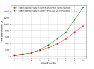
Figure 7. Time consumption for LSQ parameter estimation against object’s order by the programs using vector unit NEON on CubieBoard-3.

As one can see in both cases horizontal vectorization gives better results. And further improvements and checks will be connected only with it.

3.7.  Data Alignment

The next problem is data alignment. Old gcc compilers for armv7 required the directives explicitly showing that elements of the matrix rows and vector variables are aligned in memory at the boundaries multiple for 64 (http://infocenter.arm.com/help/index.jsp?topic=/com.arm.doc.ddi0344k/Cihejdic.html). To find out the effect of the data alignment program with horizontal vectorization was modified. Compiler’s directives __attribute__((aligned (64))) and builtin_assume aligned were addad to it.

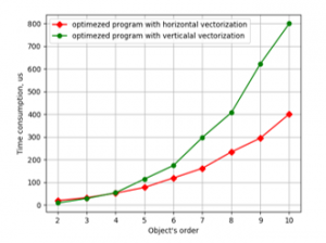
Figure 8. Time consumption for LSQ parameter estimation against object’s order by the programs using vector unit NEON on Odroid-C2.

For comparison, together with 64, the numbers 8, 16, 32 and 128 were used for alignment. Running these programs along with the program without alignment directives has shown that there is no any difference between their time consumption. That means that modern gcc compiler makes data alignment without the additional directives.

3.8.  Working with the Leftovers

The next problem one always meets while working with the vectorization is leftovers. ARM NEON vector register holds 4 single precision floating point numbers. The matrices sizes in real tasks are not multiple to 4, so the leftovers which can’t be loaded into the vector register directly must be processed in some manner. Two ways to solve this problem are suggested (https://community.arm.com/developer/ip-products/processors/b/processors-ip-blog/posts/coding-for-neon—part-2-dealing-with-leftovers). The first is to process the leftovers as non-vector data. And the second is to extend matrices to the sizes multiple to 4 and fill the edges with the zeros. The second way is considered to be faster because the vector’s processing is not interrupted with the non-vector operations.

In our case using extended matrices makes the code more sophisticated. Function for parameter evaluation takes two additional parameters and intermediate matrix S, holding informational and covariance square matrices side by side must be filled and processed in a not obvious way. As a result, the code of the function is tightly coupled with the rest of a program.

To avoid such a problem, the third way to solve leftovers problem were suggested. In this case function for parameter evaluation has local floating point arrays with the sizes equal to 4. The leftovers are loaded into these arrays before the main cycle of processing and the arrays are processed after the main cycle. These local vectors are extending each row of the matrix in a turn. As a result, all specific features connected with the vectorization are hidden within the function.

All three programs with different ways of solving the leftovers problem were checked for time consumption. The results are presented in Figures 9 and 10 for CubieBoard-3 and Odroid-C2 correspondingly.

Plots in Figures 9 and 10 show that variant with the local vectors is the worst from the point of view of time consumption, and the best is variant with the extended matrices. The difference for the object’s order from 4 to 6 is about 50% for armv8 processor and 75% for armv7. This difference is significant, so using extended matrices for the solving of leftovers problem must be recommended.

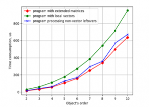
Figure 9. Time consumption for LSQ parameter estimation against object’s order by the programs using vector unit NEON and different ways of leftovers handling on CubieBoard-3.

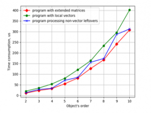
Figure 10. Time consumption for LSQ parameter estimation against object’s order by the programs using vector unit NEON and different ways of leftovers handling on Odroid-C2.

3.9.  Compare of all Results Obtained

All experimental data received in this work are presented in Table 2.

Types of the programs: 1 – QR-decompozition and dgels form lapack library; 2 – QR-decompozition and lsqsolve form gsl library; 3 – direct realization with the double precision numbers; 4 – direct realization with single precision matrices; 5 – direct realization with single precision matrices and multithreading; 6 – optimized function code; 7 – optimized function code and multithreading; 8 optimized function code with horizontal vectorization; 9 – optimized function code with vertical vectorization; 10 – optimized function code with horizontal vectorization and extended matrices; 11 – optimized function code with horizontal vectorization and non-vector leftovers.

Table 2. Time Consumption in μs for LSQ Parametrical Identification on Single-Board Computers CubieBoard-3 and Odroid-C2 for different Types of the Programs

Type	Object’s order
	2		3		4		5		6		7		8		9		10
CubieBoard-3
1	675,8		675.0		765.4		897,4		1086,1		1250,7		1568,6		1873,9		2255,9
2		295.6		399.3		447.3		565.0		736.3		999.8		1399.4		1728.7		2228.7
3		64.7		198.3		243.2		452.7		765.3		1259.5		1915.6		2852.7		3925.8
4		37.5		92.3		191.4		355.8		596.5		981.2		1377.6		2125.9		2943.5
5		440.3		442.8		510.3		564.7		710.7		885.3		1270.5		1746.3		2100.6
6		18.8		50.5		110.5		215.2		348.6		545.3		828.2		1160.9		1551.4
7		419.0		440.4		461.9		483.3		592.3		718.2		915.9		1086.5		1329.3
8		29.5		59.8		109.5		175.7		272.3		384.7		540.6		746.7		944.2
9		16.5		52.7		98.3		207.5		350.6		543.8		746.6		1135.2		1518.2
10		13.02		31.8		56.0		104.8		156.5		250.7		339.8		497.4		636.3
11		14.9		39.8		60.8		127.1		167.3		294.3		357.7		567.0		670.1
Odroid-C2
1	200.0		222.7		251.0		295.0		357.3		436.3		542.3		669.7		827.0
2		111.3		130.0		163.7		211.7		280.0		370.0		487.3		639.7		894.0
3		23.7		57.6		121.0		231.6		391.3		655.0		1031.7		1432.3		2007.3
4		24.0		57.0		120.0		226.7		383.0		595.7		884.3		1243.7		1771.0
5		543.3		547.0		627.7		819.3		925.3		1266.7		1478.3		1955.0		2422.3
6		17.0		40.3		84.3		162.3		269.0		417.0		616.7		882.4		1203.4
7		254.6		271.0		281.7		304.0		330.0		418.7		462.0		548.0		633.4
8		19.3		32.0		52.0		77.3		119.0		161.7		233.7		294.7		401.0
9		9.0		28.7		53.7		114.3		174.0		297.7		407.0		622.0		800.0
10		10.7		22.7		31.7		54.3		81.3		126.3		166.7		241.0		307.5
11		12.7		27.33		33.0		70.7		84.3		155.7		173.0		286.6		312.5

As Table 2 shows, the measures taken to optimize the code of function for LSQ parameter estimation of the object of control have allowed to reduce time consumption in 4.7 times for the processor armv7 and in 3.5 times for armv8 for the objects with the order from 4 to 6. Such significant productivity-increasing may allow to widen substantially the area of utilization of the adaptive digital controllers.

The sourse code of the programs tested in this article is available for free downloading under GPL license (https://github.com/basv0/lsq_armv7).

4. Conclusion

Wide using of the microprocessors systems that may provide high quality of technical objects control is restrained with the complexity of parameters estimation of these objects. As a result, the adaptive control may take more time than the technological process allows in hard real-time systems. This conclusion follows from the results of time consumption comparison for LSQ parameter estimation by the programs using function dgel from the linear algebra library lapack, function lsqsolve from scientific library gsl and functions for matrix multiplication and inversion. The tests show that direct realization of the matrix operations is more preferable for the tasks of not big dimensions and that using a single-precision floating-point variable instead of double precision ones does not decrease the calculations accuracy for the objects with the order less than 10.

Applying multi-threading showed that it gives productivity-increasing only for the objects with the order higher than 7 while in practice objects with the order between 2 and 6 are mainly met. Increasing productivity in the whole range from 2 to 10 may be achieved by the code refactoring and using intrinsic functions for the vector computations.

An optimized function using horizontal vectorization and extended matrices with the dimensions multiple by 4 has shown the best results. And this function is recommended for practical utilization despite the fact that matrix extension makes the code more sophisticated.

Conflict of Interest

The authors declare no conflict of interest.

1. V.V. Olonichev, B. A. Staroverov and M. A. Smirnov, “Optimization of Program for Run Time Parametrical Identification for ARM Cortex Processors,” 2018 International Conference on Industrial Engineering, Applications and Manufacturing (ICIEAM), Moscow, Russia, 2018, pp. 1-5. doi: 10.1109/ICIEAM.2018.8728595.
2.  K. Astrom and B. Wittenmark, Computer Controlled Systems. Prentice-Hall, Inc., 1984.
3.  R. Izerman. Digital Control Sytems. Springer-Verlag, Berlin, Heidelberg, New York, 1981.
4.  L. Ljung, System Identification: Theory for the User. Prentice-Hall, 1987.
5. Z. Tan, H. Zhang, J. Sun et al., “Research on Identification Process of Nonlinear System Based on An Improved Recursive Least Squares Algorithm”, Proceedings of the 31st Chinese Control and Decision Conference, CCDC 2019 8832530, pp. 1673-1678.
6. M. Arehpanahi, H R. Jamalifard, “Time-varying magnetic field analysis using an improved meshless method based on interpolating moving least squares”, Iet Science Measurement Technology, vol. 12, no. 6, pp. 816-820, May. 2018.
7. H. Li, J. Zhang, J. Zou, “Improving the bound on the restricted isometry property constant in multiple orthogonal least squares”, IET Signal Processing, vol. 12, no. 5, pp. 666-671, Apr. 2018.
8. V. Skala, “A new formulation for total Least Square Error method in d-dimensional space with mapping to a parametric line ICNAAM”, 2015 AIP Conf. Proc.1738, pp. 480106–1-480106–4, 2016.
9. H. Leslie, Handbook of Linear Algebra. – CRC Press, 2013.
10.  C.F. Jeff Wu, Michael S. Hamada Experiments: Planning, Analysis, And Optimization. Wiley, New Jersey, 2009.
11. B.A. Staroverov, V.V. Olonichev and M.A. Smirnov, “Optimal samplinig period definition for the object identification using least squares method”, Vestnik IGEU, vol 1, pp 62-69, 2014. (article in Russian with an abstract in English)
12.  W. Press, S. Teukolsky, W. Vetterling, and B. Flannery, Numerical Recipes in C: The Art of Scientific Computing. Cambrige University Press, Cambridge, New York, Port Chester, Melbourne, Sydney, 1992.
13. U. Drepper. What Every Prorgammer Shoud Know About Memory. https://www.akkadia.org/drepper/cpumemory.pdf.
14. B. Stroustrup, The C++ Programming language. Addison-Wesley, 1997.

(Click Here)

(Click Here)