1. Introduction

People who dispose of their domestic wastewater directly to the river are still found around the world. It has a high potentiality to increase pollution in the river. Then, the water quality in the river will be decreased. Hence, wastewater treatment is needed to reduce the pollutant in the wastewater before it is disposed of.  Many countries have been developing wastewater treatment plants (WWTP) to reduce the negative impacts of the wastewater they produced. Commonly, a WWTP was built with components of an inlet section at the beginning of the process, facultative ponds, maturation ponds, and outlet section [1]. To optimize the pollutant reducing on facultative ponds, many researchers have been developed some mathematical models to analyze the physical, biological and chemical processes on these ponds during the treatment. In the biological process, the organic material is decreased during a natural process which utilizes the bacteria and algae in the wastewater [2]–[4].

In mathematical theories, many mathematical models are useful to analyze some phenomena which will produce some results to be used for mitigation, optimization, evaluation, etc. One of the most useful mathematical models is the partial differential equation. For example, an elliptic partial differential equation was used to solve a production planning problem [5], a partial differential equation model was formulated for infrared image enhancement [6], and a mathematical model was applied for inflammatory edema formation [7]. The more special mathematical model in a class of partial differential equations is an equation for the advection-dispersion phenomenon. There were many pieces of researches conducted to solve and to apply the advection-dispersion model. For examples, an advection-dispersion rule was applied for analyzing of transport of leaking CO2-saturated brine along a fractured zone [8], a fractional advection-dispersion model was applied for hillslope tracer analysis, and a 3D advection-dispersion model was used to analyze the distribution of dissolved oxygen in a facultative pond [9]. The analytical solution of a partial differential equation is commonly not easy to find. Therefore, many researchers are more prefer to the numerical method to solve. Special for the advection-dispersion model, some numerical methods were developed such as random lattice Boltzmann method [10], Haar wavelets coupled with finite differences [11], unified transform/Fokas method [12], a numerical method based on Legendre scaling functions [13] and many more. Each of these methods had some superiority and weakness. Furthermore, a mathematical model contains some parameters in the equation. To determine the value of these parameters, parameter estimation is needed to be performed.

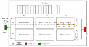
Figure 1: Sewon Bantul wastewater treatment plant [19]

Special for a partial differential equation, to be considered well to observe the modeled phenomenon, a parameter estimation process is needed to obtain the best parameter value to represent the phenomenon. There are many methods to be able to perform parameter estimation from classic methods like least square to some new methods like multi-parametric programming [14] and novel mixed artificial neural network [15]. Many researchers have been conducted some researches for parameter estimation process which have been applied for many problems like Ornstein–Uhlenbeck process [16], plasmonic QED problem [17], and gravitational waves problem [18].

In this research, we conduct a study of parameter estimation on a BOD degradation mathematical model for a two-dimensional differential equation based on the advection-dispersion model for a facultative wastewater stabilization pond. To obtain the best parameter, we use the BOD observation data taken in the Sewon wastewater stabilization pond located in Bantul, Yogyakarta, Indonesia.

2. Material and Method

The methodology used in this research is explained as follows. First, we explain the WWTP that we observed. The sample data of the BOD concentration used in the parameter estimation process were observed in Sewon WWTP located in Bantul, Yogyakarta province, Indonesia. The scheme of this WWP is illustrated in Figure 1.

This WWTP’s layout can be separated into three main parts that are inlet section, facultative ponds section, maturation ponds section, and an outlet section. These facultative ponds are connected as illustrated in the figure where the size of each facultative pond is around (77 x 70 x 4) m³. The sampling point of this research is explained in Figure 2. The used method to test the BOD concentration in the wastewater sample is APHA.AWWWA.WEF 5190 B-2012.

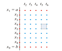
Figure 2: BOD sampling points

2.1.  Assumptions

The governed differential equation in this research is working under the following assumptions:

• The observation data were collected in Sewon WWTP in the sunny season. We assume the achieved parameter is suitable for the sunny season.
• The governed differential equation contains only two dimensions i.e. x-direction and y-direction. We omit the depth parameter and assume the BOD concentration is uniformly distributed in the depth dimension.
• Dispersion constant in the x and y direction are assumed to be identic in the horizontal direction.
• We observe only the BOD degradation in the facultative ponds. We omit the treatment on the maturation pond.

The governed differential equation used the following symbols:

i	:	index of sampling point coordinate in the x-direction
j	:	index of sampling point coordinate in the y-direction
x	:	sampling point coordinate in the x-direction
y	:	sampling point coordinate in the y-direction
	:	dispersion constant in the x or y direction
	:	BOD concentration on sampling point (i,j) at observation time instant n (ML-3)
	:	step length of observation sampling point in the x-direction
	:	step length of observation sampling point in the y-direction
	:	step length step of observation time instant
	:	observation data value of BOD concentration at sampling point (i,j) at observation time instant n (ML-3)
u	:	velocity of the flow rate of the wastewater in the x-axis direction (LT-1)
v	:	velocity of the flow rate of the wastewater in the y-axis direction (LT-1).

 2.2.  Mathematical Model

The BOD degradation process can be illustrated in Figure 3. The velocity of the flow rate of the wastewater in the x-axis direction is u (LT^-1) whereas notation v is the velocity of the flow in the y-direction (LT^-1).

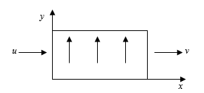
Figure 3: The BOD degradation process

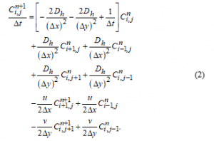
Let   be the dispersion constant in the x or y direction (L²T^-1), the parameter estimation is conducted for the following BOD degradation mathematical model in the two-dimensional equation based on the advection-dispersion process [20]:

where  is the BOD concentration (ML^-3). We assume that   which means that the dispersion constant in the x and y direction are identic as the horizontal direction denoted by  . By applying the finite difference method to solve the model numerically, we have the following solution

By simple algebraic manipulation, we have the following solution

The initial value of the model is obtained by sampling with the following method. Firstly, by using the observation BOD concentration data shown in Table 1, we have calculated the curve fitting process to obtain a BOD concentration function of the grid based on these data.

Table 1: BOD Concentration Data for initial condition curve fitting

Sampling point		y
		1	2	3	4	5	6	7
x	1	64.06	66.12	41.79	34.92	64.06	66.12	41.79
	2	34.92	64.06	66.12	41.79	34.92	37.44	40.64
	3	36.51	39.43	63.85	37.87	49.68	69.84	64.06
	4	66.12	41.79	34.92	37.44	40.64	36.51	39.43
	5	63.85	37.87	49.68	69.84	64.06	66.12	41.79
	6	34.92	37.44	40.64	36.51	39.43	63.85	37.87
	7	49.68	69.84	69.78	55.35	69.86	42.68	42.68

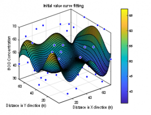
Figure 4: Initial value curve fitting

By taking , , curve fitting is resulting the following polynomial of degree 5:

which is illustrated in Figure 4. The derived initial value curve  is then used as the initial value of the BOD concentration for all sampling points in the parameter estimation calculation.

3. Results and Discussions

Let  denotes the observation data value of BOD concentration at sampling point (i,j) at observation time instant n. The governed optimization is formulated as

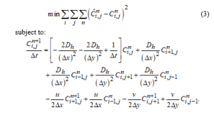
This mathematical model is explained as follows. The objective is find the best value for the parameters that will be estimated i.e. the flow rate in the x-direction & y-direction, and the dispersion constant.  The term “best” means that we want to find the value for the parameters so that the simulated data derived from   will be closest to the observation data. This can be achieved by adopting the least square theory i.e. minimizing the difference between the simulated data and the observation data of the BOD concentration value for all time instants (observation time) and for all sampling points  in the quadratic form as formulated in subject to the governed equation of the BOD concentration.

Table 2:    BOD concentration (mg/L) data for parameter estimation at time sampling 2 PM

Sampling point		y
		1	2	3	4
x	1	37.44	40.64	36.51	39.43
	2	38.32	44.24	38.38	50.97
	3	46.10	23.32	47.06	53.86
	4	55.79	47.05	23.98	64.44
	5	51.02	36.40	35.56	54.71

Table 3:    BOD Concentration (mg/L) data for parameter estimation at time sampling 7 PM

Sampling point			y
			1	2	3	4
x	1	63.85		37.87	49.68	69.84
	2	48.33		33.84	66.78	76.40
	3	49.25		26.05	43.79	42.56
	4	50.28		47.43	40.66	49.90
	5	87.05		55.08	51.34	52.44

By using the MATLAB programming language and interior-point algorithm solver, we run the parameter estimation by using the observation data. The results are the value for parameters the flow rate, dispersion coefficient in the x-direction, and dispersion coefficient in the y-direction.

Tables 2 and 3 show the BOD concentration observation data at sampling time 2 PM and 7 PM that we used to perform the parameter estimation. The optimization process or solving was performed in MATLAB R2017b on a daily used personal computer with 3.2 GHz of processor, 8 GB of memory and Windows 10 of the operating system. From the solution for , the parameter value for dispersion constant is 0.25 and the velocity of the flow rate is 0.1 for the x-direction and 0.15 for the y-direction. These values can be used in the model so that the model will give the best fit to the data with a relative error of 11.5% of the simulated data from the observed data. We argue that this relative error is acceptable which means that these results are implementable. These parameter estimation results, then, can be used to estimate the dynamics of the BOD concentration in the corresponding facultative domestic wastewater ponds via the governed differential equation .

According to the fact that the more the observation data are used, the better the estimated parameters’ value are achieved. This means that derived parameters’ value in this research might be improved by the policy maker if more observation data are available to compute although it will be costly. Moreover, time of sampling is also affecting the estimated parameter. Then, the time for collecting the observation data would be better with different conditions such as various weather. Hence, the policy maker is suggested to collect the data with multiple observations so that the estimated parameters would be better.

4. Concluding Remarks

We have considered the parameter estimation for a two-dimensional advection-dispersion mathematical model using BOD concentration data at Sewon wastewater facultative ponds located in Bantul, Yogyakarta, Indonesia. The parameters that we estimated are the flow rate in the two directions (x-direction and y-direction) and the dispersion constant. The parameter estimation process was modeled as a quadratic optimization problem in which the objective is finding the best parameter for the model and observation data using the least square scheme. We have achieved the best parameter for them with a relative error of 11.5%.

In our future works, we will develop the model for the three-dimensional case so the depth of the water will be included in the model. Furthermore, the other models for other biological/chemical processes such as chemical oxygen demand (COD), dissolved oxygen (DO), plankton, and sediment analysis are interesting to study.

{Gurauskiene, 2006, Eco-design methodology for electrical and electronic equipment industry}

Conflict of Interest

The authors declare no conflict of interest.

Acknowledgment

This research is supported by DRPM KEMENRISTEKDIKTI INDONESIA under PDUPT research grant 2018.

1. S. Sunarsih, P. Purwanto, and W. S. Budi, “Mathematical modeling regime steady state for domestic Wastewater Treatment facultative stabilization ponds,” J. Urban Environ. Eng., vol. 7, no. 2, pp. 293–301, 2013, doi: 10.4090/juee.2013.v7n2.293301.
2.  S. Kayombo, T. S. A. Mbwette, A. W. Mayo, J. H. Y. Katima, and S. E. Jorgensen, “Diurnal Cycles of Variation Physical-Chemical Parameters in Waste Stabilization Ponds,” Ecol. Eng., vol. 18, no. 1, pp. 287–291, 2002.
3.  Beran and Kargi, “A dynamic mathematical model for waste water stabilization ponds,” Ecol. Modell., vol. 181, no. 1, pp. 39–57, 2005, doi: 10.1016/j.ecolmodel.2004.06.022
4. L. Puspita, R. E., and S. I. N.N., “Lahan Basah Buatan di Indonesia. Wetlands International Indonesia Programme,” 2005.
5.  D. Covei and T. A. Pirvu, “An elliptic partial differential equation and its application,” Appl. Math. Lett., vol. 101, p. 106059, 2020, doi: 10.1016/j.aml.2019.106059.
6. D. N. Liu, R. Hou, W. Z. Wu, J. W. Hua, X. Y. Wang, and B. Pang, “Research on infrared image enhancement and segmentation of power equipment based on partial differential equation,” J. Vis. Commun. Image Represent., vol. 64, p. 102610, 2019, doi: 10.1016/j.jvcir.2019.102610.
7. R. F. Reis, R. W. dos Santos, B. M. Rocha, and M. Lobosco, “On the mathematical modeling of inflammatory edema formation,” Comput. Math. with Appl., 2019, doi: 10.1016/j.camwa.2019.03.058.
8. N. Ahmad, A. Wörman, X. Sanchez-Vila, and A. Bottacin-Busolin, “The role of advection and dispersion in the rock matrix on the transport of leaking CO2-saturated brine along a fractured zone,” Adv. Water Resour., vol. 98, pp. 132–146, 2016, doi: 10.1016/j.advwatres.2016.10.006.
9.  Sunarsih, D. P. Sasongko, and Sutrisno, “Numerical Solution of a 3-D Advection-Dispersion Model for Dissolved Oxygen Distribution in Facultative Ponds,” E3S Web Conf., vol. 31, 2018, doi: 10.1051/e3sconf/20183103006
10.  A. A. Hekmatzadeh, A. Adel, F. Zarei, and A. Torabi Haghighi, “Probabilistic simulation of advection-reaction-dispersion equation using random lattice Boltzmann method,” Int. J. Heat Mass Transf., vol. 144, p. 118647, 2019, doi: 10.1016/j.ijheatmasstransfer.2019.118647.
11.  S. Haq, A. Ghafoor, and M. Hussain, “Numerical solutions of variable order time fractional (1+1)- and (1+2)-dimensional advection dispersion and diffusion models,” Appl. Math. Comput., vol. 360, pp. 107–121, 2019, doi: 10.1016/j.amc.2019.04.085.
12.  F. P. J. de Barros, M. J. Colbrook, and A. S. Fokas, “A hybrid analytical-numerical method for solving advection-dispersion problems on a half-line,” Int. J. Heat Mass Transf., vol. 139, pp. 482–491, 2019, doi: 10.1016/j.ijheatmasstransfer.2019.05.018.
13.  H. Singh, R. K. Pandey, J. Singh, and M. P. Tripathi, “A reliable numerical algorithm for fractional advection–dispersion equation arising in contaminant transport through porous media,” Phys. A Stat. Mech. its Appl., vol. 527, p. 121077, 2019, doi: 10.1016/j.physa.2019.121077.
14.  E. Che Mid and V. Dua, “Parameter estimation using multiparametric programming for implicit Euler’s method based discretization,” Chem. Eng. Res. Des., vol. 142, pp. 62–77, 2019, doi: 10.1016/j.cherd.2018.11.032.
15.  X. Hou, J. Yuan, C. Ma, and C. Sun, “Parameter estimations of uncooperative space targets using novel mixed artificial neural network,” Neurocomputing, 2019, doi: 10.1016/j.neucom.2019.02.038.
16.  Y. A. Kutoyants, “On parameter estimation of the hidden Ornstein–Uhlenbeck process,” J. Multivar. Anal., vol. 169, pp. 248–263, 2019, doi: 10.1016/j.jmva.2018.09.008.
17.  H. R. Jahromi, “Parameter estimation in plasmonic QED,” Opt. Commun., vol. 411, no. August 2017, pp. 119–125, 2018, doi: 10.1016/j.optcom.2017.11.020.
18. A. Błaut, “Parameter estimation accuracies of Galactic binaries with eLISA,” Astropart. Phys., vol. 101, pp. 17–26, 2018, doi: 10.1016/j.astropartphys.2018.04.001.
19.  Sunarsih, Widowati, Kartono, and Sutrisno, “Mathematical Analysis for the Optimization of Wastewater Treatment Systems in Facultative Pond Indicator Organic Matter,” E3S Web Conf., vol. 31, no. 05008, pp. 1–3, 2018, doi: 10.1051/e3sconf/20183105008
20. Sunarsih, S. Dwi P, and Sutrisno, “Mathematical Model of Biological Oxygen Demand in Facultative Wastewater Stabilization Pond Based on Two-Dimensional Advection-Dispersion Model,” Am. J. Eng. Res., vol. 5, no. 11, pp. 1–5, 2016.

(Click Here)

(Click Here)