1. Introduction

Deep learning as a promising field has been quickly involving during last years. Artificial neural networks, which are cornerstone of this field, have proven to achieve overwhelming results in many disciplines. Computer vision is one of such area, where deep learning techniques are being used for solving variety of tasks. Me and my colleagues were working on a particular computer vision task in the past. Back then, we solved the problem by analytic method with use of standard computer vision functions.  Recently we decided to solve the same task by using deep learning techniques and compare the results. These objectives will be described in this paper, which is an extension of work originally presented in proceedings of the International Carpathian Control Conference 2019 [1].

Computer vision belongs to technologies in which deep learning techniques are widely used nowadays. Some of applications are for example image recognition, image processing [2], object detection [3], solving style transfer problem [4]. We cannot omit image classification problem [5], which is the issue of this paper.

Our classification problem is binary, i.e., the developed software must assign one of only two classes to the provided input data. In this particular case we are classifying kind of timber load stored on trucks. The classification should lead to a improve safety check of trucks heading into paper mill MONDI SPC, a.s. in Ruzomberok.

Similar problems of image classification have been solved in the past by applying supervised machine learning algorithms, which is the case of the article focused on classifying agricultural landscapes algorithms [6]. Next article solves the problem of cloud detection, that is binary classification problem, with use of large-scale gaussian processes classifier [7]. Next study shows a classification of heat emitting object with use of Convolutional Neural Network [8]. Network of such kind is also used in this work.

2. Recording Trucks

Before entering the paper mill MONDI SPC, each truck loaded with wood logs has to pass a safety check. For this purpose, a unique gate equipped with a set of 2D lidar scanners and a group of cameras has been developed and installed. Functionality and design of this gate are described in detail in the older article [9].

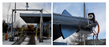Figure 1: The scanning gate (left) with detail on a camera (right).

Software executing the safety inspection of trucks use point cloud that represent a surface of each truck. These point clouds are obtained by the set of scanners while trucks are passing through the gate. The algorithm for safety check is universal for all kinds of timber load. We have an idea that can lead to improve success rate of the inspection, if we use a specific algorithm for relevant kind of timber storage.

But for that, we need to classify kind of wood storage of each truck, before running one of specifics inspection algorithm. This classification is the main goal of both original and this article. For this purpose, we can use the installed cameras, which serves now only for recording and storing an evidence of incorrectly loaded trucks.

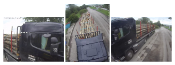Figure 2: Pictures of a truck from all three cameras.

3. Classification with use of Computer Vision Technology

The original article describes how we solved this classification problem with use of analytic functions belonging to the computer vision technology. These functions are described in detail in the book [10]. A final classification result of individual truck was determined by mean results of two classification methods.

3.1.  Top View Classification

First method works with images taken by a camera mounted on the top of the scanning gate. At the beginning of the recognition algorithm, the important area of taken image (highlighted by the blue quadrangular on the left part of Figure 3) is converted by perspective transformation into simulation of top view. Then the image is converted into grayscale one, on which the Canny algorithm for finding edges is applied.

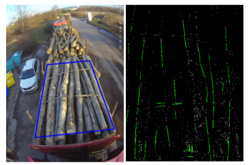Figure 3: Important area of image (left) and final image with founded lines [1].

Then lines are detected by use of Hough algorithm (see right part of Figure 3). Direction of those lines shows a type of wood storage.

3.2.  Side View Classification

This method uses images taken by cameras mounted on both sides of the scanning gate. Principle of this method is to find cross-sections of wood logs in truck’s images. When they appear in significant percentage of image’s area, then a truck is classified as transversely loaded one.

At first, via perspective transformation, an important part of an image is converted into a side view simulation. The perspective transformation is done due to easier wood logs’ cross-sections detection when they transform from shape of ellipses to more or less circular shape.

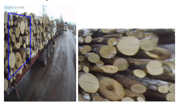Figure 4: Important area of image (left) and its perspective transformation into simulation of side view [1].

Then threshold is applied to find cross-sections of wood logs. Pure wood (cross-sections of wood logs) occur in variations of yellow color, from light to dark yellow. Whereas, tree bark (cylindrical surface of wood logs) occur in shades of brown or gray color. This feature is used in image processing to detect cross-sections of wood logs. Pixels belonging to cross-sections of wood logs are detected by applying threshold that define if pixels are within the range of yellow colors in HSV color spectrum (see Figure 5).

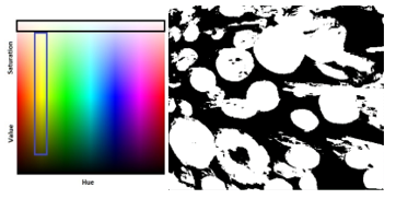Figure 5: HSV color spectrum with marked ranges of yellow color (left) and threshold of both color ranges merged together on side view image (right)

At first, the algorithm looks for cross-sections of wood logs separately on both images of thresholds of yellow color, and later on merged one.

The erode function is called on the threshold images repeatedly with different number of iterations. At first, the erode function with relatively large amount of iterations is called to split and detect bigger blobs. Afterwards, the detected blobs are subtracted from the threshold original image, and the erode function with less amount of iterations is executed to find small blobs as well.

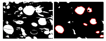Figure 6: Threshold of one of yellow colour (left) and its blob detection (right)

Detected blobs found on all three threshold images are approximated to circles. Those circles are drawn, into the image of its original perspective transformation, for better visualization (see Figure 7).

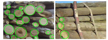Figure 7: Founded cross-sections of wood logs on transversely loaded truck (left) and on longitudinally loaded one (right) [1].

As you can see, cross sections are also detected on images of trucks with longitudinal kind of timber load. But, to classify a truck as a transversely loaded one, areas of the cross-sections must occupy significant part of the image’s total area.

4. Classification with Use of Deep Learning Technology

Image classification is one of the problems where deep learning really excels. The high success of neural networks in the field of computer vision is achieved especially thanks to convolutional layers, which works similar as human cortex. [11].

Despite long training time, neural networks are very fast and effective when they are already deployed to solve a specific task. Our image classification problem belongs to family of supervised learning. Neural networks of this group can be very accurate if the training dataset is huge and heterogenous, because in that case they learn a more general pattern [12]. Unfortunately, our dataset is rather small due to the fact, that transversely loaded trucks are extremely rare.

We had pictures of only 412 transversely loaded trucks at disposal. On the other hand, a list with records of longitudinally loaded trucks was massive. Even though, we used only 724 of these to keep moreover balanced datasets of both classes. The input data were divided into three groups. First one was used for training a neural network, second one was dedicated for validating the neural network during training, and last group was reserved for final testing of trained network.

Table 1: Distribution of input data into datasets.

	train	validation	test
longitudinal	406	156	162
transverse	231	89	92

Speed of trucks moving through the scanning gate is between 5 and 10 km/h. The cameras have a frequency of only one record per a second. Each camera takes on average 8 pictures of a truck during its scanning. Since we are using 3 cameras, each truck is represented by 24 pictures on average. The images of trucks are taken with a relatively high resolution of 2048 x 1536 pixels by the left and the right camera. Resolution of the top camera is the same, but swapped in axes, so its value is 1536 x 2048 pixels. All input images are resized to 512 x 512 pixels before entering the neural network. This action makes both evaluation and especially training phase significantly faster. The input images that are fed into the neural network, have three channels, that represent RGB color format.

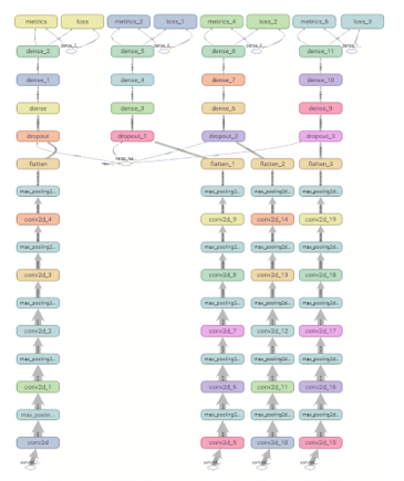Figure 8: The graph of used architecture.

The architecture of used neural network is based on VGG-19 model [13]. After using this model architecture to our classification dataset, we have done some experiments with the model configuration and slightly change its architecture. Final model is sequential, rather deep and consist of five convolutional layers. Every convolutional layer use ReLU (Rectified Linear Unit) as an activation function [14], and their kernels have a shape of 3 x 3. The number of filters increases with the depth of the model. First convolutional layer has only 32 filters, second one is made up from 64 filters, third and fourth layer have the same amount of 128 filters, and the last convolutional layer consists of 256 filters. After each of these convolutional layers, a max pooling operation, with pooling size of 2 x 2, is executed.

Then the model is flattened, and dropout function with rate of 0.5 is activated. In the end of the model are three densely connected layers. The number of units per layer is decreasing with depth from 1024 via 512 to 1. First two of these densely connected layers use ReLU activation function, whereas the last layer rely on Sigmoid activation function.

The neural network was trained for 120 epochs. The training has been done with RMSprop optimizer with 0.0001 learning rate. Choosing the hyper-parameters of the network have been done based on papers [15, 16]. Accuracy of the network was verifying on the validation dataset during training. As we can see from Figure 8, the validation accuracy stopped to follow the growing tendency of the training accuracy around 100^th epoch. After that point the network started to memorize input data rather than finding a better classification pattern.

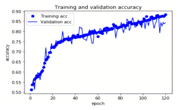Figure 9: Training the network.

After initial training, a new neural network was trained with only a hundred epochs to avoid overfitting [17]. To combat overfitting, we used the techniques described in [18, 19], which help us to choose the best elements of model dealing with that problem, and set their parameters. These techniques were proven, via comprehensive experiments, to increase the model’s classification success rate on new data. This final network was later examined on the testing dataset. The final classification accuracy achieved a result of 84.926 %, which is a great outcome received from our limited training dataset. With use of larger training dataset, we could achieve even greater success rate.

Although we tried to solve this task by training many different neural networks architectures with convolutional layers, the one described in this chapter has the best result.

The classification accuracy of the original paper with analytic approach has only slightly better result, that reached to 85,086 %. While maintaining almost identical classification accuracy, the new method is few times faster and need less computing energy.

5. Conclusion

The classification accuracy achieved by the trained convolutional neural network is 84.92%. This number is accuracy of an individual truck’s image. When we classify a truck according to a mean result of all its images, we can reach up to 97.88% success rate.

This classification problem has already been solved in the original paper by analytic methods with use of computer vision technology. Back then we achieved similar result of 98% success rate.

Classification approach of this paper uses artificial neural network, and as such, it is more reliable in bad weather and light conditions. For example, snowing, raining, cloudy weather, or darkness at night, can lead to huge unreliability of analytic approach of the original paper, since it depends on finding yellow colour of wood log cross-sections. On the other hand, actual solution can be reliable even in those bad conditions, when the images of the training dataset include images with these situations.

Even though actual solution has not brought much better result, it is far faster and more energy efficient solution than the original one. The big future potential is by combining these two methods. The determining if a truck is longitudinally or transversely loaded will reach almost a hundred percent certainty by that. Then, we can upgrade the actual software for truck’s safety inspection to work for a specific kind of timber load, and by that the safety check will be more precise.

Conflict of Interest

The authors declare no conflict of interest.

Acknowledgment

This work was supported by the European Regional Development Fund in the Research Centre of Advanced Mechatronic Systems project, CZ.02.1.01/0.0/0.0/16_019/0000867 within the Operational Programme Research, Development and Education and the project SP2020/57 Research and Development of Advanced Methods in the Area of Machines and Process Control supported by the Ministry of Education, Youth and Sports.

1.  J. Sikora, D. Fojtík, J. Czebe and M. Mihola, “Storage kind recognition of truck’s timber load”, 2019 20th International Carpathian Control Conference (ICCC), Krakow-Wieliczka, Poland, 2019, pp. 1-4.
   https://doi.org/10.1109/CarpathianCC.2019.8766049
2.  M. Jurek and R. Wagnerová, “Frequency Filtering of Source Images for LASER Engravers”, 2019 20th International Carpathian Control Conference (ICCC), Krakow-Wieliczka, Poland, 2019, pp. 1-5.
   https://doi.org/10.1109/CarpathianCC.2019.8766050
3. S. Kanimozhi, G. Gayathri and T. Mala, “Multiple Real-time object identification using Single shot Multi-Box detection”, 2019 International Conference on Computational Intelligence in Data Science (ICCIDS), Chennai, India, 2019, pp. 1-5.
   https://doi.org/10.1109/ICCIDS.2019.8862041
4. L. Gatys, A. Ecker and M. Bethge, “Image Style Transfer Using Convolutional Neural Network”, 2016 IEEE Conference on Computer Vision and Pattern Recognition (CVPR), Las Vegas, USA, 2016, pp. 2414-2423. https://doi.org/10.1109/CVPR.2016.265
5. H. R. Roth et al., “Anatomy-specific classification of medical images using deep convolutional nets”, 2015 IEEE 12th International Symposium on Biomedical Imaging (ISBI), New York, NY, 2015, pp. 101-104.
   https://doi.org/10.1109/ISBI.2015.7163826
6. D. C. Duro, S. E. Franklin, M. G. Dubé, “A comparison of pixel-based and object-based image analysis with selected machine learning algorithms for the classification of agricultural landscapes using SPOT-5 HRG imagery”, 2012, Remote Sensing of Environment, vol. 118, pp. 259-272. https://doi.org/10.1016/j.rse.2011.11.020
7.  P. M. Álvarez, A. P. Suay, R. Molina and G. C. Valls, “Remote Sensing Image Classification With Large-Scale Gaussian Processes”, 2018, IEEE Transactions on Geoscience and Remote Sensing, vol. 56, pp. 1103-1114. https://doi.org/10.1109/TGRS.2017.2758922
8. A. D. Algarni, “Efficient Object Detection and Classification of Heat Emitting Objects from Infrared Images Based on Deep Learning”, 2020, Multimedia Tools and Applications, pp. 1-24. https://doi.org/10.1007/s11042-020-08616-z
9. F. David, P. Petr, M. Miroslav and M. Milan, “Scanning of trucks to produce 3D models for analysis of timber loads”, 2016 17th International Carpathian Control Conference (ICCC), Tatranska Lomnica, Slovakia, 2016, pp. 194-199. https://doi.org/10.1109/CarpathianCC.2016.7501092
10.  G. R. Bradski, Learning OpenCV, Sebastopol: O’Reilly, 2008.
11.  W. Rawat, Z. Wang, “Deep Convolutional Neural Networks for Image Classification: A Comprehensive Review”, Neural Computation, 29(9), 2352-2449, 2017. https://doi.org/10.1162/neco_a_00990
12.  F. Chollet, Deep learning with Python, Manning Publications Co., 2018.
13.  A. Koesdwiady, S. M. Bedawi, C. Ou and F. Karry, “End-to-End Deep Learning for Driver Distraction Recognition”, 2017, Image Analysis and Recognition, ICIAR 2017, Lecture Notes in Computer Science, vol. 10317, Springer, Cham. https://doi.org/10.1007/978-3-319-59876-5_2
14.  A. F. Agarap, “Deep Learning using Rectified Linear Units (ReLU)”, arxiv 2018, ArXiv: 1803.08375
15.  L. N. Smith, “A disciplined approach to neural network hyper-parameters: Part 1 — learning rate, batch size, momentum, and weight decay”, 2018, ArXiv: 1803.09820
16.  H. Wu, Q. Liu and X. Liu, “A Review on Deep Learning Approaches to Image Classification and Object Segmentation”, 2019, CMC-Computers, Materials & Continua, 60(2), 575–597. https://doi.org/10.32604/cmc.2019.03595
17.  H. Zhang, L. Zhang and Y. Jiang, “Overfitting and Underfitting Analysis for Deep Learning Based End-to-end Communication Systems”, 2019 11th International Conference on Wireless Communications and Signal Processing (WCSP), Xi’an, China, 2019, pp. 1-6. https://doi.org/10.1109/WCSP.2019.8927876
18. A. F. Kamara, E. Chen, Q. Liu and Z. Pan, “Combining contextual neural networks for time series classification”, 2020, Neurocomputing, vol. 384. pp. 57-66. https://doi.org/10.1016/j.neucom.2019.10.113
19.  L. Pan, C. Li, S. Pouyanfar, R. Chen and Y. Zhou, “A Novel Combinational Convolutional Neural Network for Automatic Food-Ingredient Classification”, 2020, Computers, Materials & Continua, vol. 62, pp. 731-746. https://doi.org/10.32604/cmc.2020.06508

(Click Here)

(Click Here)