1. Introduction

High Dynamic Range (HDR) image Tone Mapping (TM) is an interesting subject. The objective is to find a trade-off between the relevant information such as details, contrast, brightness… to be preserved or discarded in the image ensuring a good visual quality of the displayed image on Low Dynamic Range (LDR) devices that would be appreciated by observers.

Three e-books in [1], [2] and [3] fairly describe a state of the art on HDR image TM approaches. This paper just quickly reviews the developed TM strategies that caught our attention because of their performance. In [4], the TM approach uses an edge-preserving bilateral filter to decompose the HDR image into two layers: a base layer encoding large-scale variations and a detail one. Contrast is then reduced only in the first layer while the details are kept unchanged. This TM reduces the HDR contrast while preserving the image details. In [5], an adaptive logarithmic mapping method of luminance values works with the adjustment of the logarithmic basis depending on the radiance of the pixels. A subband architecture related on an oversampled Haar pyramid representation in [6], is presented. The re-scaling of subband coefficients according to a gain control function reduces the high frequency magnitudes and boosting low ones. A TM optimization approach with adjusting a histogram between linear mapping and the equalized histogram mapping in [7] is developed. Then revisited histogram equalization approaches are discussed in [8]. The modification of this approach is made with both histogram equalization and human sensitivity to the light function.

A second generation of wavelets based on the edge content of the image avoiding having pixels from both sides of an edge in [9] is proposed. A separable non-linear multiresolution approach based on essentially non-oscillatory interpolation strategy has been investigated in [10]. This work relates to the singularities such as edge points in their mathematical models preserving then the structural information of the HDR images. The results provided in [9], [10] and [11] show that the decomposition of the HDR image on different resolution levels would seem to be a good strategy.

The proposed HDR image TM approach has two main goals namely the preservation of the details that relates to multiresolution and the adjustment of the contrast that relates to perceptual linear adjustment in accordance with the LDR display devices. It is composed of four stages in Figure 1. The first one judiciously decomposes the HDR image into different subbands (section 2.1). The second one concerns the weighting strategy of the subband coefficients (section 2.2). The third one reconstructs the coarse LDR image (section 2.3). Finally the fourth one adjusts the contrast according to a perceptual linear quantizer (section 2.4). Section 3 discusses the simulation results. Section 4 concludes the paper.

2. Proposed HDR image tone mapping approach

This section concerns four stages of the proposed HDR image TM mapping approach such as decomposition, weighting, reconstruction and contrast adjustment stages.

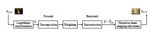
Figure 1: Diagram block of the proposed HDR image TM algorithm.

Let introduce some notations. Assume that size N^J × M^J is the original HDR image at the finest resolution level J. Define the index j which refers to the resolution level with j = 0,…, J − 1. Denote l_HDR the HDR image luminance. In the rest of this paper, the HDR image luminance is considered in the logarithm domain since it is well adapted to the human visual system. It is denoted

I^J and defined as follows I^J = {I^J(x_n,y_m) = ^log₁₀(l_HDR(x_n,y_m)) where 1 ≤ n ≤ N^J and 1 ≤ m ≤ M^J. Hence I^J(x_n,y_m) is the HDR logarithm luminance value of the pixel located at position (x_n,y_m) on the image.

2.1        First stage: HDR image multiscale decomposition

The decomposition of the HDR image consists to go from the finest resolution level J to the coarsest resolution level 1. At a given resolution level j (with 1 ≤ j ≤ J), the algorithm deals with the approximation coefficients denoted I ^j(x_n,y_k) (with 1 ≤ n ≤ N ^j and 1 ≤ k ≤ M ^j) computed at resolution level j. The approximation resolution level I ^j(x_n,y_m) is divided into 4 blocks I ^j := (I ^j−1,d_HL^j−1,d_LH^j−1,d_HH^j−1) (with LL is Low Low, LH Low High, HL High Low and HH High High) which saves into a non-redundant way. The decomposition is thus iterated on I ^j−1 until j = 1. The original HDR image I^J is then represented by 3J + 1 subbands or resolution levels IJ := (I0,dHL0 ,dLH0 ,dHH0  ,…,dHLJ−1,dLHJ−1,dHHJ−1).

2.2        Second stage: Weighting strategy of the subband coefficients

In order to reduce the dynamic range of the HDR image, the TM approach proposes to weight the approximation and detail coefficients in an appropriate way before performing the adaptive lifting scheme backward process described in section 2.3.

Denote N_l the number of resolution levels equal to J; E_a the entropy of the approximation coefficients at the coarsest resolution level (j = 1); and E_d^j the entropy of the detail coefficients at resolution level j (such as d_HL^j , d_LH^j and d_HH^j ) getting therefore N_l + 1 entropies (E_a, E_d⁰, E_d¹, …, E_d^j−1,…, E_d^Nl−1). From these entropies, positive weights smaller than one are deduced as follows:

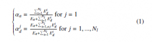
α_a (respectively ^α_d^j) is the weight associated to the approximation (respectively detail) coefficients at resolution level j = 1 (respectively j).

The coefficients of the four coarsest resolution levels are first modified according to:

The approximation subband, denoted I⁰¹, is then reconstructed (see section 2.3) and the number of levels is reduced to N_l − 1. The N_l entropies (associated to 3N_l − 2 subbands) are calculated again to update the weights α_a, α¹_d (equation (1) with N_l = N_l − 1). After that, these weights are applied on the coefficients I⁰¹,^d_HL¹ ,^d_LH¹ ,^d_HH¹ to build I⁰² as explained above. This process is iterated until N_l = 1 to reconstruct the coarse tone mapped HDR image denoted _eI_LDR^J , called coarse LDR image.

2.3        Third stage: Reconstruction of the coarse LDR image

The reconstruction is worked inversely to the decomposition stage. Assume at the resolution levels j−1, the next step consists to recover the approximation coefficients I^0j of size N ^j × M ^j using 4 weighted blocks I^0j−1, d_LH^0j−1, d_HL^0j−1 and d_HH^0j−1. The reconstruction is iterated to finally build the image I^0J later called coarse LDR image which is denoted eILDRJ .

2.4        Fourth stage: Piecewise linear perceptual quantizer

To enhance the contrast, this stage proposes to adjust locally the distribution of the coarse LDR image logarithm luminance _eI_LDR^J according to the HVS using a piecewise linear function. The _e^I_LDR^J values are first sorted and statistically classified into equal B bins defined by cutting points denoted cⁱ_uLDR. A non-uniform histogram equalization is also performed with cⁱ_nuLDR cutting points with 1 ≤ i ≤ B. The lower bound (cutting point) of each bin is then adjusted as follows:

eliLDR(1) = β(cinuLDR − ciuLDR) + ciuLDR, (3) where β is a positive parameter smaller than 1.

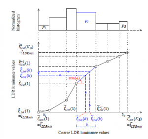
Figure 2: Piecewise linear modelization (”s-shaped” curve).

Therefore the _e^I_LDR^J values are classified into non-uniform B bins as follows:

where K_i is the number of values in the i − th bin (with 1 ≤ i ≤ B; K_i > 0) and satisfying the following relation ^P_i^B₌₁ K_i = N^J × M^J.

The ”s-shaped” TM perceptual curve, as discussed in [12] and

[13], is modelled by a piecewise linear curve on each bin (see Figure 2). Consider the i − th bin, defined by [_elⁱ_LDR(1),…,_elⁱ_LDR(K_i)], the coarse LDR values are then modeled as follows:

The parameter aⁱ is unknown and deduced so that the norm-M space error between the HDR value and its quantized version (denoted

Extending equation (7) to all bins involves the computation of a global norm-M space error Ψ deduced as follows:

Therefore the unknown parameter bⁱ is calculated as follows: bⁱ = lˆⁱ_LDR(1) − aⁱ ×_elⁱ_HDR(1) and LDR mapped values are deduced according to equation (5).

3. Simulation results

This section provides the performance of the proposed tone mapped HDR image. Simulations have been conducted under Matlab environnement using the HDR Toolbox ([1]) with 300 test HDR images. The tone mapped image quality is measured with the TMQI (ToneMapped image Quality Index) metric [14]. For lack of space, we only present the results obtained with 8 HDR images (”Anturium”, ”Small Bottle”, ”Small Office”, ”Oxford Church”, ”Memorial”, ”Light”, ”Ward Flowers” and ”Street Lamp”) with different dynamic range (or contrast ratio) from 8.7 f-stops to 18.4 f-stops.

The proposed approach is compared to: (i) Li TMO [6] with Haar multiscale; (ii) Duan [7] using β = 0.5; (iii) Fattal [9] using RBW method with parameters α = 0.8, β = 0.3, γ = 0.8;

(iv) SEP ENO-CA [10] with parameters α₁ = 0.3, α₂ = 0.7; (ii) NONSEP ENO-CA [11]; (v) TMOs in HDR Toolbox: Durand [4], Drago [5], Reinhard [15], Ward [16], Tumblin [17], Schlick [18] with the default parameters as given in the HDR Toolbox. The different parameters are chosen so as to give the best results in terms of TMQI metric in all methods.

Table 1 provides the TMQI metrics. The proposed TM approach namely ”Proposed LJ” is deployed with Biorthogonal 2.2 wavelet (bior2.2) properties, B = 256, M = 2, β = 0.25, l_LDRmax = 255, l_LDRmin = 0 and J = 1,…,5. Our approach is competitive to those developed in the literature. More the number of resolution levels increase, more the performance increase.

Figure 3 compares the visual quality of the ”Oxford Church” tone mapped image using ”Duan” method and our approach. The stained glass window at the church background presents a better contrast and details with our approach although the TQMI are identical. Figure 4 compares the ”Memorial” tone mapped image using

”Duan” and ”Fattal” methods and our approach. The details on tills (see Figure 4) and rosette (see Figure 5) are better rendered by our approach.

Figure 6 compares the visual quality of the ”Ward Flowers” tone mapped image using ”Fattal” and our approach. Some details, on flowers and rocks, are lost on ”Fattal” tone mapped image compared to our approach. Moreover, our tone mapped image if of better contrast. A similar result is provided by Figure 7 where the HDR ”Street Lamp” image has been mapped using ”SEP ENO” method and our method. The brightness of our tone mapped is better.

Figure 8 compares the visual quality of the ”small office” tone mapped image using ”Duan”, ”Fattal”, ”Li” and our approach. Compared to other tone mapped images, ”Li” tone mapped image doesn’t seem to be natural. Indeed its normalized histogram given in Figure 9 shows that the pixel grey levels are limited to 60. Some of the details from outside the office (via the window) are lost on ”Fattal” tone mapped image (brightness) contrary to our approach and ”Duan” method. Indeed the brightness on ”Fattal” tone mapped image is confirmed by the pic corresponding to a grey level equal to 255 on its normalized histogram (see Figure 9). However ”Duan” tone mapped image is a little darker (armchair, office wall) than our tone mapped image. This analysis is well supported by the normalized histograms of our approach and Duan method. The comparison of the histograms proves that our strategy stretches the too-dark areas and suppresses the too-bright areas.

The performance of our approach is confirmed on more than 300 test HDR images where the details and contrast are better represented than other competitive methods.

4. Conclusion

This paper proposed a new HDR image TM approach while preserving as much information of the HDR image as possible. This is essentially related to : (i) the weighting operation depending on the information of each subband; (ii) the adjustment of the coarse LDR image luminance distribution according to the perceptual piecewise linear function. Simulation results confirm the relevance of the proposed approach both in terms of the TMQI metric and the visual quality of the displayed image. These are results related to the advantage of using multiresolution and piecewise linear perceptual quantization.

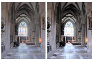
Figure 3: ”Oxford Church” HDR test image (15.5 f-stops) – Up image: proposed (5 levels, TMQI=0.986); Down image: ”Duan” (TMQI=0.987).

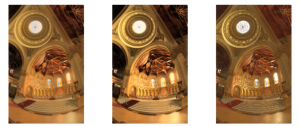
Figure 4: ”Memorial” HDR test image (18.4 f-stops) – Left image: proposed (5 levels, TMQI=0.952); Middle image: ”Duan” (TMQI=0.936); Right image: ”Fattal” (TMQI=0.928).

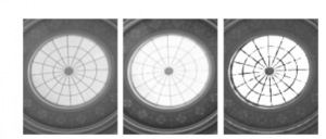
Figure 5: LDR luminance ”Rosette” zoom – Left image: proposed (5 levels, TMQI=0.952); Middle image: ”Duan” (TMQI=0.936); Right image: ”Fattal” (TMQI=0.928).

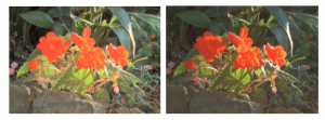
Figure 6: ”Ward Flowers” HDR test image (14.0 f-stops) – Up image: proposed (5 levels, TMQI=0.931); Down image: ”Fattal” (TMQI=0.876).

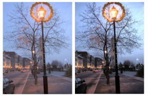
Figure 7: ”Street Lamp” HDR test image (13.8 f-stops) – Up image: proposed (5 levels, TMQI=0.912); Down image: ”SEP ENO” (TMQI=0.856).

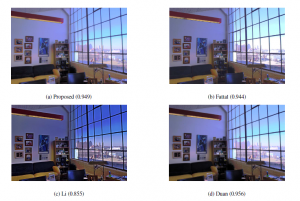
Figure 8: ”Small Office” HDR tone mapped images.

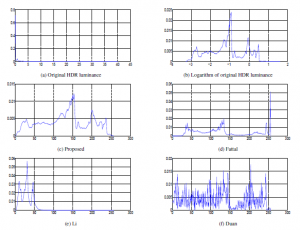
Figure 9: Normalized histograms of original ”Small Office” HDR luminance and its tone mapped images.

Table 1: Tone Mapped Image Quality Index (TMQI)

TMOs/HDRi	Anturium	Small	Small	Oxford	Memorial	Light
		Bottle	Office	Church
DR (f-stops)	8.7	16.1	16.3	15.5	18.4	17.5
Durand [4]	0.812	0.893	0.826	0.930	0.815	0.801
Drago [5]	0.875	0.802	0.801	0.815	0.801	0.801
Li [6]	0.965	0.955	0.855	0.878	0.835	0.889
Duan [7]	0.965	0.917	0.956	0.987	0.936	0.970
Fattal [9]	0.890	0.929	0.944	0.890	0.928	0.972
SEP ENO [10]	0.897	0.935	0.944	0.896	0.933	0.971
NONSEP [11]	0.939	0.874	0.936	0.821	0.833	0.933
Reinhard [15]	0.779	0.808	0.827	0.790	0.792	0.795
Ward [16]	0.807	0.784	0.776	0.818	0.796	0.790
Tumblin [17]	0.716	0.714	0.736	0.676	0.760	0.751
Schlick [18]	0.771	0.836	0.927	0.971	0.788	0.781
Proposed L1	0.947	0.864	0.935	0.955	0.919	0.955
Proposed L2	0.966	0.883	0.939	0.971	0.930	0.964
Proposed L3	0.979	0.905	0.946	0.982	0.942	0.967
Proposed L4	0.981	0.922	0.947	0.985	0.950	0.970
Proposed L5	0.983	0.934	0.949	0.986	0.952	0.970

Acknowledgment

This research is funded by Funds for Science and Technology Development of the University of Danang under project number B2019-DN02-51.

1.  Banterle, F., Artusi, A., Debattista, K., and Chalmers, A., “Advanced High Dynamic Range Imaging: Theory and Practice”, AK Peters (now CRC Press), ISBN: 978-156881-719-4 (2011).
2.  Dufaux, F., Le Callet, P., Mantiuk, R., Mrak, M., “High Dynamic Range Video 1st Edition : From Acquisition, to Display and Applica- tions”, ISBN: 9780081004128 (April 2016)
3.  Reinhard, E., Heidrich, Wolfgang., Debevec, Paul., Pattanaik, S., Ward, G., and Myszkowski, K., “High Dynamic Range Imaging 2nd Edition: Acquisition, Display, and Image-Based Lighting”, ISBN: 9780123749147 (May 2010).
4.  Durand, F., and Dorsey, J., “Fast Bilateral Filtering for The Display of High-dynamic-range Images”, ACM Transactions on Graphics (TOG)
   – Proceedings of ACM SIGGRAPH 21, pp. 257-266 (2002).
5.  Drago, F., Myszkowski, K., Annen, T., and Chiba, N., “Adaptive Log- arithmic Mapping for Displaying High Contrast Scenes”, Computer Graphics Forum 22, pp. 419-426 (2003).
6.  Li, Y., Sharan, L., and Adelson, E.H., “Compressing and Companding High Dynamic Range Images with Subband Architectures”, ACM Trans. Graph. 24, pp. 836-844 (July 2005).
7.  Duan, J., Bressan, M., Dance, C., and Qiu, G., “Tone-mapping High Dynamic Range Images by Novel Histogram Adjustment”, Pattern Recognition, vol. 43, pp. 1847-1862 (2010).
8. Husseis, A., Mokraoui, A., and Matei, B., “Revisited Histogram Equalization as HDR Images Tone Mapping Operators”, 17th IEEE International Symposium on Signal Processing and Information Tech- nology, ISSPIT (December 2017).
9.  Fattal, R., “Edge-Avoiding Wavelets and their Applications”, ACM Trans. Graph (2009).
10.  Thai, B.C., Mokraoui, A., and Matei, B., “Performance Evaluation of High Dynamic Range Image Tone Mapping Operators Based on Sep- arable Non-linear Multiresolution Families”, 24th European Signal Processing Conference, pp. 1891-1895 (August 2016).
11.  Thai, B.C., Mokraoui, A., and Matei, B., “Image Tone Mapping Ap- proach Using Essentially Non-Oscillatory Bi-quadratic Interpolations Combined with a Weighting Coefficients Strategy”, 17th IEEE Interna-tional Symposium on Signal Processing and Information Technology, ISSPIT (December 2017).
12.  Dowling, J. E., “The Retina: An Approachable Part of the Brain”, Cambridge, Belknap Press (1987).
13.  Geisler, W. S., “Effects of Bleaching and Backgrounds on the Flash Response of the Cone System”, Journal of Physiology, 312:413434 (1981).
14.  Yeganeh, H. and Wang, Z., “Objective Quality Assessment of Tone- mapped Images”, IEEE Trans. on Image Processing, vol. 22, pp. 657-667 (February 2013).
15.  Reinhard, E., and Devlin, K., “Dynamic Range Reduction Inspired by Photoreceptor Physiology”, IEEE Transactions on Visualization and Computer Graphics 11, pp. 13-24 (2005).
16.  Ward, G., Rushmeier, H., and Piatko, C., “A Visibility Matching Tone Reproduction Operator for High Dynamic Range Scenes”, IEEE Transactions on Visualization and Computer Graphics 3, pp. 291-306 (1997).
17.  Tumblin, J., and Rushmeier, H., “Tone Reproduction for Realistic Images”, IEEE Comput. Graph. Appl, pp. 42-48 (1993).
18.  Schlick, C., “Quantization Techniques for Visualization of High Dynamic Range Pictures”, In Proceeding of the Fifth Eurographics Workshop on Rendering, pp. 7-18 (1994).

(Click Here)

(Click Here)