1. Introduction

Computer vision deals with the extraction of valuable information from the contents of digital images, real-world objects, or videos. One of many problems that exists in computer vision is object recognition. The study of object recognition has been done over decades since the 1960s [1], which makes it an old task and sometimes described as a challenging task. There are two approaches in Object Recognition: Object Classification and Object Instance Recognition / Fine-Grained Recognition. Object Classification means classifying objects in general categories/class i.e. human, animal, and vehicle. While Object Instance Recognition means recognizing objects in specific categories/class i.e. book covers, DVD covers, soda cans, and canned food [2] with one or small reference images per class. Fine-Grained Recognition also means recognizing objects in specific categories/class, but with small visual differences, which needs large number of reference images per class.

This paper focuses on proposing a method for Object Instance Recognition that combines Salient Object Detection and Image Matching with Geometric Verification.

Most previous works in Object Instance Recognition are feature-based. Such works include Triplets of feature descriptors proposed by Zitnick et al. [2]. Kusuma et al. proposed Object Recognition using Weighted Longest Increasing Subsequence [3]. Xie et al. proposed Dense Feature extraction using SIFT and pose base verification [4], Best Increasing Subsequence (BIS) and image matching for Object Instance Recognition is proposed by Kusuma and Harjono [5] and the development of BIS which is Best Score Increasing Subsequence (BSIS) using SURF for feature extraction and image matching is proposed by Kusuma et al. [6]. Meanwhile, there are also deep learning methods for Object Instance Recognition, such as Held et al. proposed feed-forward neural network for a single image [7].

The most approach in Object Instance Recognition uses feature-based approach because of single image reference, and it is becoming unpopular nowadays because of deep learning. However, the performance of deep learning deteriorates when there is only a single reference image per class. This capability is still needed for certain applications such as visual search and augmented reality. Therefore, this research tries to develop better feature-based approach with the hope of improving its accuracy.

There are few reasons why feature-based is used rather than deep learning approaches in this research. One of them is because there is only one reference image per class which means deep learning approach is not suitable to use. In this research, Geometric Verification is used as a method to verify the similarity score between the reference and testing images and to increase the accuracy. Geometric Verification needs spatial locations of features, and it is produced by a feature-based approach, not by deep learning. Even though deep learning extracts local features, but the location information of the features is not preserved.

Commonly, feature-based approach extract features from the raw image, but it could waste time and unimportant features can be extracted too. Instead of extracting features from the raw image, it is beneficial to extract features only from salient image areas. There is a method called Salient Object Detection which detects noticeable or important objects in an image. It works by narrowing down which image region to be extracted, so it can be more focused and accurate only on the noticeable object in the image. Therefore, Salient Object Detection is used for masking the feature extraction.

There are many types of Salient Object Detection methods from hand-crafted to deep learning approach. Such as Salient object using shape prior extraction which proposed by Jiang et al. [8], Graph-based manifold ranking from Yang et al. [9], Contrast-based filtering from Perazzi et al. [10], Histogram-based contrast from Cheng et al. [11], and Window composition from Feng et al. [12]. But, based on our literature study, hand-crafted approaches are a bit outdated both in accuracy and processing times. Hence, recently many researchers use deep learning approach that performs well and overcomes the hand-crafted method. For example, Multi-Context Deep Learning using CNN as proposed by Zhao et al. [13]. While Li and Yu [14] proposed the Deep Contrast Network method which used CNN for extracting features efficiently and produce accurate results than other methods. Liu and Han [15] proposed a deep hierarchical saliency network. Li et al. [16] proposed a Multiscale Refinement Network (MSRNet). Wang et al. [17] used RFCN for saliency detection and Qin et al. [18] performs CNN combined with the Residual Refinement Module (RRM).

Table 1: Summary related works in Object Instance Recognition

Category	Methods	Datasets	Performance Measure (evaluation)	Results
Conventional method (Feature-based)	Image Matching, Grouping features in triplet, Geometric Hashing [2]	118 objects divided into 2: 1. Non-occluded single object 2. occluded multiple objects	ROC Curve	Detection Rate: 1. Single object: 78.8% 2. Multiple objects: 81.1%
	Image Matching and Geometric Verification using Weighted Longest Increasing Subsequence (WLIS) [3]	1. Stanford Mobile Visual Search (SMVS) 7 Categories 2.Their dataset 2 Categories 3. Images from internet: 1300 images.	1. E value = (CRR*CJR) / (1+IRR)	Average E: 1. SURF+ WLIS: > 20% better than SURF matching > 4% better than SURF+RANSAC
	Dense Feature extraction, RANSAC Pose Estimation and Multimodal Blending [4]	1. Willow 2. Challenge	1. Precision 2. Recall 3. F score	Willow & Challenge (sequentially): Precision: 0.9828, 1.000 Recall: 0.8778, 0.9977 F score: 0.9273, 0.9988
	Best Increasing Subsequence (BIS) [5]	1. Stanford Mobile Visual Search (SMVS) 7 categories. 2. Non-related images from internet	1. E measure = (CRR * CJR) / (1 + IRR)	Average E measure: SURF+BIS: 82.34% SURF+WLIS: 77.43% SURF+RANSAC Homography: 73.51% SURF Only: 53.49%
	Best Score Increasing Subsequence (BSIS) [6]	1. Stanford Mobile Visual Search (SMVS) 7 categories. 2. Non-related images taken from internet.	1. E measure = (CRR*CJR) / (1 + IRR)	Average E measure: SURF+BSIS: 86.86% SURF+BIS: 82,34% SURF+WLIS: 77,43% SURF+RANSAC Homography: 73,51%
Deep Learning	CNN model with CaffeNet architecture [7]	1. RGB-D 2. BigBird	Accuracy	Testing Accuracy: 1. Single view object during training: – Textured object: 73.8% – Untextured object: 60.0% – Overall: 63.9% 2. Object with occlusion and real background: 44.1%

This paper delivers a combination method for Object Instance Recognition that consists of Salient Object Detection, Image Matching, and Geometric Verification. The goal of this paper is to propose a new method for Object Instance Recognition that produce reliable results for the case of one reference image available per class.

2. Related Works

2.1.  Related Works of Object Instance Recognition

 Object Instance Recognition is a more refined method of object recognition that provides information about the attribute of an object such as the object’s name. There is another method which is quite like Object Instance Recognition called Fine-Grained Recognition. The difference from Object Instance Recognition is that Fine-Grained Recognition uses many training or reference images and usually employs a deep learning approach. Meanwhile, Object Instance Recognition is defined as a method that commonly uses a single reference image per class. Nowadays, Object Instance Recognition method that uses one reference image becomes unpopular. Only a few researches that explained about Object Instance Recognition, can be seen in Table 1. That is because deep learning becomes more well-known and Fine-Grained Recognition become a new challenge in recent years.

From Table 1, it can be seen that performance measurement varies because Object Instance Recognition is an old method.  However, researchers tried to show their contribution to the development of Object Instance Recognition. The same table showed that feature-based approach is more reliable than deep learning when one reference image per class is used. Deep Learning performs well when many reference images in each class are available.

2.2.  Related Works of Salient Object Detection

Salient Object Detection aims to highlight, predict and distinguish between an object of interest and its background object [19]. It works by predicting the object of interest in an image. There are many previous works in Salient Object Detection that researchers have done as seen in Table 2.

From Table 2, both Conventional and deep learning approaches are still used for Salient Object Detection. However, according to our observation, since 2015 deep learning is becoming more popular and promising to perform Salient Object Detection. It can achieve higher F-score and MAE compared to conventional methods. For example, Qin et al. [18] proposed CNN combined with residual refinement to produce an accurate saliency map. It can be seen from the result, the proposed method gets high F-score and MAE in six datasets such as SOD, ECSSD, DUT-OMRON, PASCAL-S, HKU-IS and DUTS-TE, also overcome other methods. Hence, deep learning becomes the best approach for Salient Object Detection nowadays.

3. Combination of Salient Object Detection and Image Matching

Figure 1 shows the flowchart of the combination method between Salient Object Detection [18] and Image Matching with Geometric Verification based on [6]. The process mainly divided into 5 steps: Salient Object Detection (step 1), Feature Extraction, Feature matching and pre-filtering features (steps 3-5b).  Calculating the pair score (step 6), Geometric Verification (step 7-8) and Acceptance/Rejection of the results (step 9-10). Feature extraction for the testing image is slightly different because it uses a saliency map to extract features.

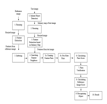Figure 1: Flowchart of the combination method

The method begins by resizing reference and testing images, while the saliency map is resized along with testing images. The feature extraction is performed directly for the reference image, which means without using a saliency map, while the testing image is used a saliency map to extract features. All feature extraction is done using the Speeded Up Robust Feature (SURF) [22]. Then, all extracted features will be indexed to ease pair candidates searching. Later, all matched pair candidates which pass the threshold will be given similarity score and then passed to Geometric Verification to verify its pairs. Geometric Verification will determine the correct pairs based on the highest similarity score between reference and testing images. To accept/reject testing images, a threshold will be used. Only when the testing image’ score is higher than the threshold, it will be accepted. In this research, Salient Object Detection is used only for the pre-processing method and image matching with Geometric Verification for the main process.

3.1.  Salient Object Detection

This research uses a Convolutional Neural Network (CNN) model for Salient Object Detection [18]. The method is called Boundary-Aware Salient Object Detection (BASNet) which is a predict-refine model. The method was chosen as the Salient Object Detection technique because it is relatively new, appearing in 2019 and provides good results. The architecture of BASNet based on [18] can be seen in Figure 2.

Table 2: Summary related works in Salient Object Detection

Author	Methods	Datasets	Performance Measure	Results
Conventional Methods	Energy minimization and combination between bottom-up saliency information and object-level shape prior [8]	2 datasets used: 1. Achanta et al. [20] 2. MSRA-B	1. F alpha 2. Boundary Box Displacement Error (BDE)	F alpha: The proposed method consistently achieves the highest F alpha on both datasets. BDE: The proposed method gets the lowest BDE (above 20 but less than 25)
	Manifold ranking [9]	3. datasets used: 1. MSRA 2. MSRA-1000 3. DUT-OMRON	1. F measure	F measure: 1. In MSRA and MSRA-1000: the method performs well to achieve the highest precision and recall. 2. DUT-OMRON: the method still performs poorly.
	Saliency filters using N-D Gaussian filtering, SLIC algorithm, K-means [10]	1. Natural images from [21]	1. F measure 2. Mean Absolute Error (MAE)	F measure: Approximately above 0.8 but less than 0.9 (only shown in the chart) MAE: In range 0.3-0.4 ( only shown in chart)
	SaliencyCut using histogram and spatial information region-based contrast [11]	3 datasets used: 1. Achanta et al. [20] 2. MSRA10K 3. THUR15K	1. F measure 2. True Positive Ratio (TPR)	F measure: Achanta dataset: above 0.9, MSRA10K: in range 0.8-0.9 (only shown in chart). TPR: Top 50 retrieval results: 78.2% and Top 100: 78.4%.
	Segment-based window composition algorithm [12]	2 datasets used: 1. PASCAL VOC 07 2. MSRA	1. Average precision.   2. F measure:	F measure: 1. MSRA: 0.82
Deep Learning	SLIC and CNN with global and coarse context [13]	5 datasets used: 1. ASD 2. SED1 3. SED2 4. ECSSD 5. PASCAL-S	1. F measure	F measure: 1. ASD: 0.9548 2. SED1: 0.9295 3. SED2: 0.8903 4. ECSSD: 0.7322 5. PASCAL-S: 0.7930
	Deep Contrast Learning based on CNN model using pixel level-segment pooling stream and CRF model [14]	5 datasets used: 1. MSRA-B 2. HKU-IS 3. DUT-OMRON 4. PASCAL-S 5. SOD	1. F measure 2. MAE	F measure: 1. MSRA-B: 0.916 2. HKU-IS: 0.904 3. DUT-OMRON: 0.757 4. PASCAL-S: 0.822 5. SOD: 0.832	MAE: 1. MSRA-B: 0.047 2. HKU-IS: 0.049 3.DUTOMRON: 0.080 4. PASCAL-S: 0.108 5. SOD: 0.126
	Global-View CNN + Hierarchical Recurrent CNN  [15]	4 datasets used: 1. ECSSD 2. MSRA10K, 3. DUT-OMRON 4. PASCAL-S	1. F measure	F measure (only shown in chart): Above 0.8 and close to 0.9: 1. ECSSD, MSRA10K Above 0.7 and less than 0.8: 1. DUT-OMRON, PASCAL-S
	Fully Convolutional Multiscale Refinement Network (MSRNet) [16]	6 datasets used: 1.MSRA-B 2.PASCAL-S 3.DUT-OMRON 4.HKU-IS 5.ECSSD 6.SOD	1. F- measure 2. Mean Absolute Error (MAE)	– MSRA-B: 0.930, 0.042 (F measure, MAE) PASCAL-S: 0.852, 0.081 DUT-OMRON: 0.785, 0.069 HKU-IS: 0.916, 0.039 ECSSD: 0.913, 0.054 SOD: 0.847, 0.112 -New dataset for salient object instances (1000 images)
	Recurrent Fully Convolutional Networks (RFCN) [17]	4 datasets used: 1. SED1 2. ECSSD 3. PASCAL-S 4. HKU-IS	1. F measure 2.Mean Absolute Error (MAE)	F measure: 1. SED1: 0.8811 2. ECSSD: 0.8713 3. PASCAL-S: 0.7784 4. HKU-IS: 0.8564	MAE: 1. SED1: 0.0750 2. ECSSD: 0.0668 3. PASCAL-S: 0.1049 4. HKU-IS: 0.0547
	CNN, Predict Module (Encoder – Decoder) and Residual Refinement Module [18]	6 datasets used: 1. SOD 2. ECSSD 3. DUT-OMRON 4. PASCAL-S 5. HKU-IS 6. DUTS-TE	1. F measure, 2. Relax F measure 3. Mean Absolute Error (MAE)	F measure, Relax F measure and MAE sequentially: 1. SOD: 0.851, 0.603, 0.114 2. ECSSD: 0.942, 0.826, 0.037 3. DUT-OMRON: 0.805, 0.694, 0.056 4. PASCAL-S: 0.854, 0.660, 0.076 5. HKU-IS: 0.928, 0.807, 0.032 6. DUTS-TE: 0.860, 0.758, 0.047

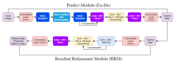Figure 2: BASNet Architecture based on [18]

The method is divided into 2 stages, predict module and Residual Refinement Module (RRM). The model uses ResNet-34 as a backbone. Predict module is designed as an encoder-decoder model, which able to capture low and high-level details at the same time. Where RRM is designed to refine the saliency map of the predicting module by learning the residuals between saliency map and ground truth. To reduce overfitting, the last layer of each decoder stage is supervised by ground truth image which inspired by Holistically Nested Edge.

Predict module consists of Encoder-Decoder parts. The encoder part has a convolution layer and six stages of basic res-block for each part. Encoder part is based on ResNet-34, but some modifications are made to the input layer, which does not have a pooling operation after the input layer and has 64 convolution filters with size 3×3 stride 1, which makes the feature map have the same resolution as the input image. The original ResNet-34 has the quarter resolution in the feature map.

To capture global information from the encoder part, a bridge is made which consists of three convolution layers with 512 dilated (dilation = 2) 3×3 filters. The decoder part almost similar to the encoder in which each stage consists of three convolution layers, Batch Normalization (BN), and ReLU activation function.

Decoder part works by concatenating feature maps of up-sampled output from the previous stage and next stage in the encoder, to achieve side-output saliency maps. The output of bridge and decoder stage is fed to 3×3 convolution layer to perform bilinear up sampling and sigmoid function. The process produces seven saliencies which has the same size with the input image’s size, where the highest accuracy of coarse maps is taken to the refinement module.

The residual refinement module (RRM) is designed as a residual block that refines the predicted coarse saliency maps. Refined saliency maps are obtained from saliency coarse map added with saliency residual map as shown in Equation (1).

Illustration of the RRM model can be seen in Figure 3. The RRM module consists of 4 stages of encoder-decoder, where each stage only has one convolution layer. Each layer has 64 filters size 3×3, batch normalization and, ReLU function. By using non-overlapping max pooling for down-sampling and bilinear interpolation for up-sampling, final saliency maps are obtained.

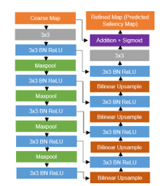Figure. 3:  Residual Refinement Module on BASNet [18]

3.2.  Image Matching and Geometric Verification using Best Score Increasing Subsequence (BSIS)

Image Matching and Geometric Verification using BSIS [6] is performed after features from testing and reference images are extracted. Features extraction will be done using Speeded Up Robust Features (SURF) [22]. It was chosen because it is relatively fast compared to other feature extraction methods. Since SURF returns features in vector forms, it is indexed using KD-Tree [23]. Indexed features from testing and reference images then enter the nearest neighbor steps, by using Euclidean distance

to find N (N=100) closest pair features. Pair features are then subjected to filtering by keeping only those with dissimilarity scores lower than the pre-filter threshold as defined in Equation (2).

where m is the mean of Gaussian distribution and K is a constant value. In this case, K = 3 with the purpose that features that are not quite potential still can be evaluated in pair verification step. Pair candidates with scores less than or equal to the threshold will be taken to the next step. Pair candidates that pass the pre-threshold will be given a pair score using Equation (3).

P_w is pair weight/score. P_QF is a point feature of testing/query image ∈ set of testing/query features. P_TF is a point feature of a training/reference image ∈ set of training/reference features. m is the mean of Gaussian distribution which calculated using median and σ is a standard deviation. After assigning a score, the verification of each pair is doing using the BSIS method. This method determines the target object based on the highest similarity score and it is proven that the method is invariant to affine transformation. Figure 4 shows illustrated Geometric Verification on BSIS. The reference and testing image in Figure 4 are used only to show how BSIS works, both images are not from the SMVS dataset.

All pair scores in Figure 4 are only illustrative which are calculated using Equation (3). Number 1-6 (under bicycle image) represents test features and 0-6 represent train features along with its feature name and features that are paired. For example, feature C is paired to two different train features (R, T) which results in two feature pairs; P5, P6.

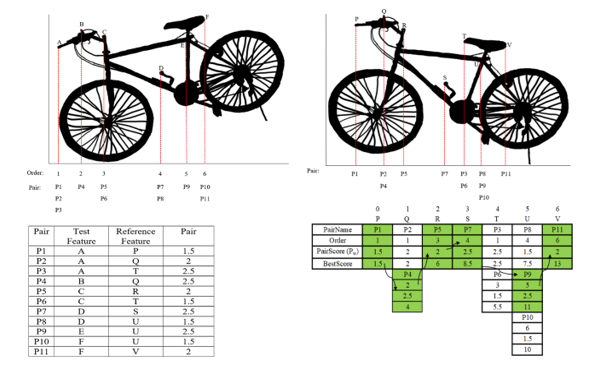Figure 4: Illustrated Geometric Verification using Best Score Increasing Subsequence. Right: Reference Image, Left: Testing Image

The best score is obtained based on the highest total similarity score and the correct sequence. The correct sequence must meet the following requirements: pair candidates must not in the same column and higher-order numbers must be chosen than the current pair candidates, not the other way around. The correct sequence according to Figure 4 is P1, P4, P5, P7, P9, P11 with total similarity score = 13. This correct sequence is obtained by performing repetition and rotation of the image, either by X-axis or Y-axis.

Acceptance or rejection of an image is based on the similarity score. If the score is higher than the threshold as shown in Equation (4), the image is accepted or matched with the reference image or otherwise.

Where m defines mean of Gaussian Distribution and σ defines the standard deviation from the top 60 best results for the query or test images. While L is a parameter value of the Gaussian Threshold for each category of SMVS dataset. L value is determined for each category based on experimental results; therefore, L value may be different for each category.

4. Experimental Results

4.1.  Datasets

This research used two datasets: SMVS (Stanford Mobile Visual Search) dataset [24] and 1300 negative images taken from the internet. Salient Object Detection is evaluated using the SMVS dataset, while Object Instance Recognition is evaluated using the SMVS dataset and 1300 negative images. SMVS dataset used has 7 out of  8 categories. Only 7 categories of SMVS dataset were used so the results could be compared with previous methods that also use 7 categories, especially BSIS which is the benchmark in this research. The categories are Book Covers, Business Cards, CD Covers, DVD Covers, Museum Paintings, Print, and Video Frames. Each category has 91-101 classes and each class has 5 images (1 image for reference and 4 images for testing). Negative images are images that are not included in the training/reference images. The purpose to use negative images is to evaluate our method whether it could correctly recognize images that are not included in the training/reference images. Details of the SMVS dataset can be seen in Table 3.

Table 3: Details of SMVS Dataset

Category	Class	Training image	Testing Image
Book Covers	101	101	404
Business Cards	100	100	400
CD Covers	100	100	400
DVD Covers	100	100	400
Museum Paintings	91	91	364
Print	100	100	400
Video Frames	100	100	400

4.2.  Implementation and Experimental Setup

The Salient Object Detection method used comes from [18], Fine-tuning were performed to their pre-trained model. Using the SMVS dataset, the model is tuned so it fits the 7 categories. We took 1 image per class in 7 categories, total 692 images are used for training images. During the training, based on BASNet each image is resized to 256 x 256 and randomly cropped to 224 x 224 and for testing, each input image is first resized to 256 x 256 then resized back to the original size of the input image.

For Object Instance Recognition, BSIS was modified so that it can be used in this research [6]. Both reference and testing images are resized into 640 x 640 for feature extraction. The methods were implemented on Pytorch 1.0.0 and A four-core PC with AMD Ryzen 1500x 3.5GHz (with 8GB RAM) and a GTX 1050TI GPU for Salient Object Detection and Visual Studio 2019 (C# language) for Best Score Increasing Subsequence (BSIS).

4.3.  Evaluation Metrics

This section will explain about evaluation techniques used in this research which combines two methods: Salient Object Detection and Object Instance Recognition.

Salient Object Detection is evaluated using two methods: F_β measure and Mean Absolute Error (MAE). F_β measure is a standard way to evaluate predicted saliency map. F_β measure is obtained from precision and recall which is calculated by comparing the saliency map to the ground truth mask. F_β measure is calculated using Equation (5).

β is set to = 0.3  to weight the precision more than the recall [25]. The maximum F_β (maxF_β) of each category SMVS is reported in this paper.

Like F_β measure, Mean Absolute Error (MAE) also a standard way to evaluate saliency maps. MAE denotes the average absolute difference per pixel between the saliency map and ground truth. The formula of MAE can be seen in Equation (6).

where H denotes height, W denotes the width of the image. S (x, y) represents the x-y coordinate of the saliency map and G (x, y) represents the x-y coordinate of the ground truth mask.

        Meanwhile, Object Instance Recognition is evaluated using E measure Firstly, E measure is introduced by [3] which aims to calculate the result between positive and negative images. In E measure, three main values are used to calculate the value of E:

• Correct Recognition Rate (CRR) is a number of the correct and accepted images divided by total positive images.
• Incorrect Recognition Rate (IRR) is a number of positive images that incorrectly recognized divided by total positive test images.
• Correct Rejection Rate (CJR) is a number of negative images that are rejected divided by total negative test images.

Therefore, E measure can be calculated using Equation (7).

4.4.  Results

4.4.1.  Salient Object Detection

This section shows the result of maxF_β and MAE Salient Object Detection in the SMVS dataset. The results are based on 50 test images are taken from each category in the SMVS dataset. There are no criteria when selecting 50 images, the images are taken randomly, and each test image only represents one class. There are 350 test images for seven categories of SMVS dataset. Since the SMVS dataset did not provide the ground truth image, we need to make the ground truth mask of the test images.

Table 4: maxFβ and MAE score of seven categories SMVS dataset for 50 images

Category	maxFβ	MAE
Book Covers	0.928	0.083
Business Cards	0.993	0.012
CD Covers	0.937	0.070
DVD Covers	0.977	0.017
Museum Paintings	0.985	0.020
Print	0.979	0.031
Video Frames	0.935	0.084

Table 4 shows the score of maxF_β (higher is better) and MAE (lower is better). The bolded number indicates the top three performances. The highest maxF_β and the lowest MAE are possessed by Business Cards. This may be influenced by several factors, such as business card object’s is easy to spot in the image because there are no other objects that attract attention in the background of the same image and business cards does not have many form variations (which may be quite similar to train image). While CD Covers, Video Frames, and Book Covers respectively become the three lowest categories. Although the MAE of Book Covers is better than Video Frames, the difference is only 0.001. Therefore, Book Covers and Video Frames can be categorized equivalent in terms of MAE. Reasons for these three categories could be due to the wide variety of test images, there are other interesting objects in the background of the same image, and during the training process may be few numbers of training images/iterations could affect the result. However, the results can be categorized as a good result. Figure 5 shows the Example of the input image, ground truth image, and results from the saliency map in the SMVS dataset.

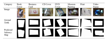Figure 5: Example of Image, Ground Truth (GT) and Saliency Map of SMVS Dataset

• Object Instance Recognition using BSIS

This section presents the result of the proposed method. Compared to other existing methods, our proposed methods can overcome others. The results are shown by the E score in Table 5.

In Table 5, results for WLIS, BIS, and BSIS are taken from the paper [6]. Our results can be seen in the fourth column “BSIS with Salient Object Detection”. Bold indicates E scores higher than others. Overall, our work overcomes WLIS and BIS in every category of the SMVS dataset. While in BSIS, our result still cannot surpass E score BSIS in the Print category. Although most of the high score is owned by BSIS with Salient Object Detection, the average E score does not significantly increase with only 1.92% higher from 86.86% to 88.78%.      

Table 5: E score of BSIS, BSIS with Salient Object Detection and other existing methods

Category	Methods
	WLIS[3]	BIS[5]	BSIS[6]	BSIS with Salient Object Detection
Book Covers	87.52%	95.22%	96.98%	97.70%
Business Cards	62.83%	64.34%	70.69%	79.35%
CD Covers	83.49%	87.00%	91.15%	93.30%
DVD Covers	88.70%	94.76%	97.19%	97.88%
Museum Paintings	74.47%	86.69%	86.93%	89.48%
Print	48.60%	52.25%	66.60%	63.99%
Video Frames	96.43%	96.10%	98.52%	99.75%
Average	77.43%	82.34%	86.86%	88.78%

5. Conclusion

In this paper, we proposed a combination method for Object Instance Recognition. The method is a combination of Salient Object Detection and Image Matching with Geometric Verification using BSIS. Based on the experimental result, the fine-tuned model Salient Object Detection performs well on the SMVS dataset. Maybe, better improvement for F-measure and MAE can be achieved by adding more training images and increase the iteration number. While in Object Instance Recognition, the proposed method that is combination of Salient Object Detection and Image Matching can be concluded improve the E score but not significant, the increase is only 1.92% higher than the previous method BSIS without Salient Object Detection.

From this research, it can be concluded that the proposed combination method can improve the E score in SMVS dataset, but not significant. Many factors could influence the results such as, using Salient Object Detection in the SMVS dataset is not too beneficial because the object is clear and the background images are clean, i.e. there are no background objects that are interfering with the foreground object.

1.  A. Andreopoulos and J. K. Tsotsos, “50 Years of object recognition: Directions forward,” Comput. Vis. Image Underst., vol. 117, no. 8, pp. 827–891, 2013.
2.  C. L. Zitnick, J. Sun, R. Szeliski, and S. Winder, “Object Instance Recognition Using Triplets of Feature Symbols,” Technology, pp. 1–15, 2007.
3.  G. P. Kusuma, A. Szabo, L. Yiqun, and J. A. Lee, “Appearance-Based Object Recognition Using Weighted Longest Increasing Subsequence,” in International Conference on Pattern Recognition, 2012.
4.  Z. Xie, A. Singh, J. Uang, K. S. Narayan, and P. Abbeel, “Multimodal Blending for High-Accuracy Instance Recognition,” 2013 IEEE/RSJ Int. Conf. Intell. Robot. Syst., 2013.
5.  K. D. Harjono and G. P. Kusuma, “Object Instance Recognition Using Best Increasing Subsequence,” 2016 11th Int. Conf. Knowledge, Inf. Creat. Support Syst., 2016.
6.  G. P. Kusuma, K. D. Harjono, and M. T. D. Putra, “Geometric Verification Method of Best Score Increasing Subsequence for Object Instance Recognition,” 2019 6th Int. Conf. Inf. Technol. Comput. Electr. Eng., pp. 1–5, 2019.
7.  D. Held, S. Thrun, and S. Savarese, “Deep Learning for Single-View Instance Recognition,” no. March, 2015.
8. H. Jiang, J. Wang, Z. Yuan, T. Liu, and N. Zheng, “Automatic salient object segmentation based on context and shape prior,” Procedings Br. Mach. Vis. Conf. 2011, pp. 110.1-110.12, 2011.
9.  C. Yang, L. Zhang, H. Lu, X. Ruan, and M. H. Yang, “Saliency detection via graph-based manifold ranking,” Proc. IEEE Comput. Soc. Conf. Comput. Vis. Pattern Recognit., pp. 3166–3173, 2013.
10.  F. Perazzi, P. Krahenbuhl, Y. Pritch, and A. Hornung, “Saliency Filters: Contrast Based Filtering for Salient Region Detection,” IEEE Conf. Comput. Vis. Pattern Recognit., 2012.
11.  M.-M. Cheng, N. J. Mitra, X. Huang, P. H. S. Torr, and S.-M. Hu, “Global Contrast Based Salient Region Detection,” {IEEE} Trans. Pattern Anal. Mach. Intell., vol. 37, no. 3, pp. 569–582, 2015.
12.  J. Feng, Y. Wei, L. Tao, C. Zhang, and J. Sun, “Salient Object Detection by Composition,” in International Conference on Computer Vision, 2011.
13.  R. Zhao, W. Ouyang, H. Li, and X. Wang, “Saliency Detection by Multi-Context Deep Learning,” IEEE Conf. Comput. Vis. Pattern Recognit., pp. 1265–1274, 2015.
14.  G. Li and Y. Yu, “Deep Contrast Learning for Salient Object Detection,” IEEE Conf. Comput. Vis. Pattern Recognit., pp. 478–487, 2016.
15.  N. Liu and J. Han, “DHSNet: Deep Hierarchical Saliency Network for Salient Object Detection,” IEEE Conf. Comput. Vis. Pattern Recognit., pp. 678–686, 2016.
16.  G. Li, Y. Xie, L. Lin, and Y. Yu, “Instance-Level Salient Object Segmentation,” in IEEE Conference on Computer Vision and Pattern Recognition (CVPR), 2017, pp. 247–256.
17.  L. Wang, L. Wang, H. Lu, P. Zhang, and X. Ruan, “Salient Object Detection with Recurrent Fully Convolutional Networks,” IEEE Trans. Pattern Anal. Mach. Intell., 2018.
18.  X. Qin, Z. Zhang, C. Huang, C. Gao, M. Dehghan, and M. Jagersand, “BASNet: Boundary-Aware Salient Object Detection,” in Conference on Computer Vision and Pattern Recognition (CVPR), 2019, pp. 7479–7489.
19.  J. Zhang, F. Malmberg, and S. Sclaroff, Visual Saliency: From Pixel-Level to Object-Level Analysis, 1st ed. Springer International Publishing, 2019.
20.  R. Achantay, S. Hemamiz, F. Estraday, and S. Süsstrunky, “Frequency-tuned salient region detection,” 2009 IEEE Comput. Soc. Conf. Comput. Vis. Pattern Recognit. Work. CVPR Work. 2009, vol. 2009 IEEE, no. Ic, pp. 1597–1604, 2009.
21.  D. Martin, C. Fowlkes, D. Tal, and J. Malik, “A Database of Human Segmented Natural Images and its Application to Evaluating Segmentation Algorithms and Measuring Ecological Statistics,” in Proceedings Eighth IEEE International Conference on Computer Vision. ICCV 2001, 2001.
22.  H. Bay, T. Tuytelaars, and L. Van Gool, “SURF: Speeded-Up Robust Features,” in European Conference on Computer Vision, 2006, pp. 404–417.
23.  J. L. Bentley, “Multidimensional Binary Search Trees Used for Associative Searching,” Commun. ACM, vol. 18, no. 9, 1975.
24.  V. R. Chandrasekhar et al., “The stanford mobile visual search data set,” Proc. Second Annu. ACM Conf. Multimed. Syst. – MMSys ’11, p. 117, 2011.
25.  R. Achantay, S. Hemamiz, F. Estraday, and S. Süsstrunky, “Frequency-tuned salient region detection,” 2009 IEEE Comput. Soc. Conf. Comput. Vis. Pattern Recognit. Work. CVPR Work. 2009, no. Ic, pp. 1597–1604, 2009.

(Click Here)

(Click Here)