1. Introduction

Atmospheric aerosol concentrations have attracted increasing worldwide attention during the past years due to its effect on human health and the environment [1]. According to The World Health Organization (WHO), it is estimated that around 7 million people die every year due to air pollution [2]. Therefore, having real time information about air pollutants concentration could help in controlling air pollution and preventing health issues that are related to its effect [3].

Recently, many researchers have put forward efforts to improve the approach to air pollution prediction. The methods of predicting air pollution concentration, in general, fall into two categories: deterministic and statistical. Deterministic models simulate the spatiotemporal distributions of air pollutants at different scales and directions by using statistical methods [4, 5, 6]. Deterministic models use physics and chemical reactions in the atmosphere to model emission and transformation of air pollutants. These models are considered theoretical models that are based on sophisticated priori knowledge, inconsistent and limited data [7, 8].

Statistical models use statistics-based models to predict air pollutants concentrations. Regression, Time Series, and Autoregressive Integrated Moving Average (ARIMA) are the most common statistical approaches that are used in the environment science prediction [9, 10, 11]. Due to a non-linear relationship between air pollutant concentration and metrological parameters, advanced statistical approaches based on machine learning algorithms are needed such as ensemble learning algorithms [12] and recurrent neural network (RNN) [13].

RNN is a type of artificial neural network that has a cycle within the network graph which maintains the internal state. RNN is able to predict in sequence prediction problems that involve a time component. This makes it suitable to be applied in applications that utilize a sequence of observations over time, such as Biomedicine, Meteorology, Genomics and more. Within the environmental engineering field, RNN has been used to predict air pollution. Due to its influence of more than one metrological parameter (such as temperature, pressure, humidity, etc), the air pollution prediction is considered as a multivariant time-series prediction problem.

Long Short-Term Memory Unit (LSTM), is a state-of-the-art model of RNN that is recently used to predict air quality [14, 15]. Many variants of RNN have been developed with different characteristics. They include GRU (gated recurrent unit), Vanilla LSTM and more.

Several attempts have been made to better predict accuracy of time-series forecasting problems using RNN models. In order to obtain advantages of several recurrent neural network models, a combination of different models can be applied. The ensemble of multi-models is a suitable solution [16]. Combining a different number of recurrent neural network models can enhance forecasting performance and increase accuracy. Conversely, ensemble methods may lead to an increase in the cost of computation time that is needed to train multi-models based on the number of models utilized. This paper will highlight some of the challenges that are faced in the application of different recurrent neural networks for forecasting applications, especially air pollution forecasting in terms of performance and accuracy. The contributions of this paper are summarized as follow:

1. Summarize the state-of-the-art recurrent neural network models that have been applied in the application of forecasting air pollution.
2. Study of challenges of designing a recurrent neural network model.
3. Recommend some of the issues that will have to be tackled before designing recurrent neural network.
4. Present the advantages of using ensemble method to enhance forecasting performance.
5. Analyze and compare the performance of different ensemble recurrent neural network for time-series forecasting applications.
6. Propose a framework for time-series forecasting based on the using of ensemble technique.

The reminder of this paper is organized as follow: Section 2 will give a brief description of the air pollution concept along with the methods that are used for its prediction. Section 3 will provide details of recurrent neural networks, some of its variations and the challenges of its design. Section 4 will present the ensemble model concepts design. Section 5 will propose the framework for time-series forecasting. Section 6 will offer the conclusion.

2.  Air Pollution

In urban cities, air pollution is one of the most significant environmental concerns that has a great impact on health and the ecosystem. Air pollution effects air quality and is one of the causes for various diseases such as heart disease, chronic obstructive pulmonary disease, acute and chronic respiratory conditions and cancers [2]. Air pollutants can be formed due to a chemical reaction with other pollutants and atmospheric physics. The prediction of air pollutants can enhance the scientific understanding of air pollution and provide valuable information concerning the contribution of each pollutant toward the cause of air pollution [17-21]. This information will provide public authorities the time to manage pollution so as not to exceed acceptable levels.

According to World Health Organization (WHO), 7 million people die every year due to air pollution. PM2.5 (particulate matter less than 2.5 micrometers in diameter) is the air pollutant that is the most likely cause of the majority of death and disease. Ozone is another pollutant that is the cause of some of the major respiratory diseases. Oxides of Nitrogen (NOx), a major contributor to ozone, is also linked to significant health risks [2].

Due to its harmful effect on human health, some major cities, such as Los Angeles and New York, have identified air pollution as one of the main health dangers [22], and so, air pollution technology has become an important topic for the creation of smart environment and for the delivery of clean air for citizens.

Many researches have been conducted over past years to propose and develop a predictive model for the concentration of air pollutants. The accuracy of these models differs based on the methods that have been employed. However, it is still a challenge to develop an accurate predictive model for the concentration of air pollution due to the existence of many factors that influence its performance [23].

The methods of predicting air pollution can be classified into two categories [24]: deterministic and statistical methods. Deterministic methods simulate the physical and chemical transformation, emission and desperation of pollutants in terms of metrological variables in the atmospheric physics. Statistical methods apply statistic-based models to predict future air pollution from historical data. These methods involve a time-series analysis. It includes linear regression [25], the autoregressive moving average (ARMA) method [26], the support vector regression (SVR) method [27], the artificial neural network (ANN) method [28], and hybrid methods [29] to understand the relationship between the concentration of air pollutants and metrological variables.

Artificial neural network is a machine learning technique that provides convincing performance in the field of time-series forecasting and prediction. ANN can incorporate complex non-linear relationships between the concentration of air pollutants and metrological variables. Various ANN structures have been developed to predict air pollution over different study areas, such as neuro-fuzzy neural network (NFNN) [30], Bayesian neural network [31] and Recurrent neural network (RNN) [32, 33]. RNN has been applied in many studies involving time-series prediction, such as traffic flow prediction [34] and wind power prediction [35]. In the area of air pollution, RNN is suitable to capture the dynamic nature of the atmospheric environment [24]. It can learn from a sequence of inputs to model the time-series of air pollution.

3. Recurrent Neural Network

Recurrent Neural Network is a type of machine learning algorithm that was developed in 1980 [36]. It is the neural network model that is most likely used for time-series forecasting problems. RNN are designed with memory to remember things from past occurrences that can be useful for prediction of the future events. Its structure has a recurrent edge between hidden nodes. So, RNN not only uses input data but also uses the output of the previous steps to make current predictions.

Figure 1 shows a simplified structure of RNN with one input layer and one output layer. The input can be considered as a sequence of vectors through time t such as {xt, xt+1, xt+2, …} where xt = (x0, x1, x2, …, xN). the input units are fully connected with hidden units, where the connections are defined by weights value. The hidden layer contains units that are connected to each other with recurrent connection through time to define memory of the system.

The hidden units are connected with output units. As the inputs are sequential through time, the feedback loop forms the cyclical structure that allow a sequential input to loop in the layer. This means that the output of step t-1 is fed back to the network to influence output of step t [36].

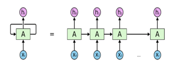Figure 1: Recurrent Neural Network [36]

RNN can deal with sequential input and produce sequential output. The input is considered internally dependent where RNN can capture this dependency with time relation. Some application areas of RNN with sequential data include handwriting recognition [37], video captioning [38] and music composition [39].

To learn input-output relationship, RNN uses a nonlinear activation function at each unit. Nonlinear activation function is more powerful than linear activation function. It is differentiable and can deal with nonlinear boundaries.

RNN uses Backpropagation algorithm during learning process to update and adjust network weights [40]. As the updating follows the modifications during feedback process, it is commonly referred to as the backpropagation through time (BPTT). The BPTT works backward through the network layer by layer from the network output, updating the weights of each layer according to the layer’s calculated portion of the total output error. The weights are changing with proportion to the derivative of error with respect to the weights value, this includes that nonlinear activation function is differentiable. The changing of weights represents distance between current output and desired target.

Computing error derivative through time is done at each iteration to make a single update and capture dependencies between parameters in order to optimize results. Updating weights back into every timestep takes time and slows learning.

Two main issues may occur during weights update, exploding gradient and vanishing gradient. The exploding gradient happens when the algorithm assigns a high importance to the weights. On long sequence data, RNN gradients may explode as weights become larger with increasing of gradients during training. While vanishing gradients happens when the partial derivation of error is very small, multiplying its value with learning rate to update weights will not be a big change compared with previous iteration. This cause network to iteratively learn with no much changes as memory will hardly learn correlation between input and output and thus will ignore long term dependencies.

Several solutions have been proposed in the literature to overcome vanishing and exploding gradient. The most popular are Long short-term memory (LSTM) and Gated recurrent unit (GRU) which are explained next in this section.

Long short-term memory (LSTM) [41] is a variant of RNN that is used to solve the problem of short-term memory. LSTM uses gate mechanism that control the flow of data. The gate decides whether the coming input data is important to be kept in the memory or not. RNN keeps all the data during the learning process, even if the update is very small and not important (vanishing problem). The gates in LSTM store important data even if it is long for a prolonged period of time. This makes LSTM capable of learning long-term dependencies as a default. Repeating modules structure in LSTM is different than RNN. Each module has four interacting layers with a unique method of communications, as shown in Figure 2.

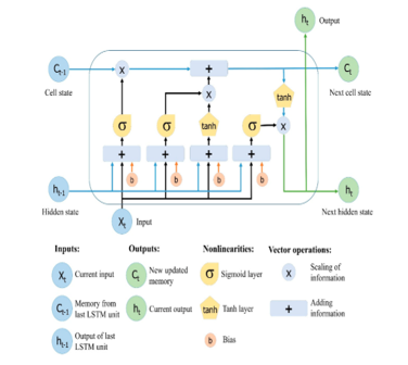Figure 2: LSTM structure [42]

The LSTM structure consists of memory block called cells. The cell state and hidden states are transferred to the next cell. The cell state is the data flow that allows data to be transferred unchanged to the next cell. Cell state is the long-term memory. The gates are similar to layers that perform some matrix operations to add or remove data from the cell state. Gates control the memorizing process to avoid long term dependency problem. The input gate and forget gate manage cell state.

Gated recurrent unit (GRU) is another variant of RNN [43]. GRU have faster learning process than LSTM and with fewer gates and shorter memory. GRU has two gates, update gate and reset gate, with no output gate in contrast to LSTM. Update gate controls information flow from the previous activation and the addition of new information. Reset gate is inserted into the candidate activation. GRU outperforms LSTM for music and speech applications [44].

The inputs to RNN, LSTM and GRU are one-dimensional vectors. Bidirectional LSTM process sequential input with opposite direction with two hidden states that accept past data and future data [45]. Bidirectional LSTM is suitable with the application where current information is influenced by previous and future inputs such as speech [46].

Choosing the appropriate algorithm among RNN versions is dependent on the problem domain and requirements. The main factor here is to improve the learning process by obtaining a satisfiable accuracy that has a low error rate and reasonable speed up. The model performance of all RNN versions is dependent on the optimization of the network hyperparameters. The hyperparameters define the neural network architecture and determine the behaviour of the algorithm for the given dataset. They include: activation function, number of hidden layers, number of neurons in each layer, sequence length, learning rate, weights initialization, number of epochs, batch size, dropout rate and feature extraction.

Finding the optimal selection for each parameter for the optimization of network performance is a challenge. The most widely applied method for the selection of hyperparameters of a given algorithm on a given dataset are grid search and random search. In grid search, all possible combinations of parameters are tested. This method is time consuming and dependent on several hyperparameters that are essential for it to be optimal. As more parameters are included, the complexity increases. However, random search chooses a random point from the parameters space, and unlike grid search which considers all possible combinations, random search is much faster with less complexity.

Selecting hyperparameters is a data driven method that requires fitting the model and validating it on the existing data, which make the process expensive [47, 48].

Table 1 summarizes the neural network hyperparameters that influence network performance, along with a list of some methods that are used to set each one up.

Choosing the value of each hyperparameter depends on the problem and its domain. Machine learning problems can be classified into two categories: classification and regression; similar for the activation function. Some of the activation function are used for classification problems, such as softmax, and some are used for regression problems, such as ReLu. The distribution of the dataset aids in determining the activation function that effect the behavior of the training.

Table 1: neural network hyperparameters

Hyperparameter	Description	Methods
Activation function	Mathematical function used to generate output value	Sigmoid, ReLu, softmax, tanh
Optimization algorithm	The mathematical method used to update network weights to make accurate prediction and minimize loss function value	Gradient decent, AdaGrad, Adam, RMSProp
Loss function	The difference between model prediction values and actual, which is needed to predict	Mean square error, mean absolute error, cross entropy
Number of hidden layers	Number of hidden layers in the network that add a hierarchy learning capacity	Experimental
Number of neurons	Number of neurons at each layer that affects the learning capacity of the network	Experimental
Learning rate	Steps forward to move weights in the direction opposite to gradient	Experimental
Weights initialization	Initial weight values	Normal distribution, uniform distribution, identity matrix, random orthogonal matrix
Number of epochs	Number of iterations	Experimental
Batch size	Number of input samples, how often to update weights of the network	Experimental
Dropout rate	Number of connections to be dropped during training	Randomly
Feature extraction	Set of features used to train predictive model	Filter method, wrapper method, embedded method

Neural networks are trained using stochastic gradient descent, which maps inputs to outputs from training data. This requires the choosing of a suitable loss function for the given problem. The model, with a given set of weights, makes prediction and, error is calculated; the optimization algorithm then updates the weights so that the following evaluation will reduce the error.

Depending on the properties of the problem and the goals of designed model, an optimization algorithm and loss function can be selected that guarantee a satisfiable result.

The number of hidden layers, number of neurons in each layer, batch size and number of epochs can influence the performance of training in terms of speedup and increase complexity. For problems where speed is not important, fixing parameters to increase accuracy by selecting large values, as needed, may not be a big issue. Determining the optimal number is a large task, and it can be done by repeating the same experiment and calculating statistics summary, which can then be compared with each configuration.

The learning rate communicates to the optimizer of the learning algorithm as to how far to move the weights in response to the estimation error after weight updating. If it is small, the training is more reliable, but more time will be needed. If it is high, then training may not converge or may even diverge. Learning rate is one of the most important parameters that need to be tune correctly before training the neural network, and its value has a great influence on the training results and network performance. Learning rate value ranges between 0.0 and 1.0.

The weight of the neural network should be initialized to a small random value. By doing this, the hidden layer will acquire a chance to generate different signals. If the weights are initialized with the same value, then the hidden layer will generate same signal. The initialization should be asymmetric (different) so that the model can find different solutions to the problem. Choosing the method that is best able to initialize the weight of the network in a way that would enhance its performance is a challenge and considered as an entire field of study.

Dropout is a technique proposed by Srivastava, et al. in 2014 to select randomly neurons to be dropped during training [49]. After each epoch, selected dropout neurons do not contribute to the activation on the forward pass, and their weights are not updated in the backward pass.

Neuron dropping during the training signifies that other neurons weights are tuned to specific features of the dataset, and this provide some specialization to training data. Selecting dropout neurons randomly gives the network a better generalization, since the un-dropped neurons will need to handle the representation to make prediction of the missing neurons, which will be led to a reduction in the overfitting of the training data and enhance performance.

Feature extraction means to select those features from the dataset that are more related to the problem and effect the training results. Irrelevant, unneeded and redundant features can be eliminated from the data before training the model. Thus, those features cannot influence the accuracy of the model. Small number of features reduces the complexity of the model, and vice versa.

Selecting the optimal value for each network hyperparameters in a way that it will enhance the performance of the model is mainly dependent on the problem domain and its dataset. The greater the parameters of hyperparameters that need to be tuned, the greater the time needed to tune them. It is preferred to select the minimum number of subsets for the hyperparameters that will influence the performance of the related problem.

3.1.  Recurrent Neural Network for Forecasting Air Pollution

There are many studies that applied the recurrent neural network for forecasting application. In this section, we will introduce some of these works that have specifically focused on the prediction of air pollution. along with a summary of the tuned hyperparameters for each, the main contributions of each one, the conducted results and pitfalls of each work are summarized in Table 2.

Lim, et al. used recurrent neural network to design a model that predicts various types of air quality over three different area in Daegu Metropolitan City, Korea. The author examined the model over different time steps and found that the error is small when the length of input data is about 30 or lower [50]. Authors [51] developed a forecasting model by combining convolution neural network (CNN) and Long Short-Term Memory to predict particulate matters (PM2.5). Li, at al., proposed a novel long short-term memory neural network extended (LSTME) model that inherently considers spatiotemporal correlations for air pollutant concentration prediction [24]. TAO, et al., proposed a model that combines RNN and CNN for air pollution forecasting [52]. Sun, et al., proposed a spatial temporal PM2.5 concentration prediction framework using GRU, which is an extension of RNN [53]. Athira, et al., proposed a deep learning architecture that consists of input layer, a recurrent structure with three neural networks: RNN, LSTM and GRU, and a prediction layer to predict PM10 [54]. Xayasouk, et al., combined RNN with GRU to predict PM10 and PM2.5 in Seoul, South Korea.  The proposed model can forecast the concentration of the future 20 days based on previous history data [55].

Brian, et al., used RNN with LSTM to predict an 8-hour average surface ozone concentration based on hourly air monitoring station measurements [56]. Rao, et al., proposed an RNN-LSTM framework for quantification and prediction of air quality [57]. Zhao, et al., applied RNN to forecast daily Air Quality Classification (AQC) in three different cities in the United States, including Los Angeles (LA), Houston (HOU) and Atlanta (ALT) [58]. Karimian, et al., implemented three machine learning approaches: Multiple Additive Regression Trees (MART), a Deep Feedforward Neural Network (DFNN) and a new hybrid model based on long short-term memory (LSTM) to forecast PM2.5 concentration over different time length. LSTM achieved best results [59]. Septiawan and Endah proposed the implementation of Backpropagation Through Time (BPTT) algorithm on three models of RNN: Elman RNN, Jordan RNN, and a hybrid network architecture to predict air pollutant concentration [60].

3.1.1  Discussion about Related Works

From the above-mentioned related works, several recommended points can be concluded:

1. Each region has its specific features that are distinct from one another. The air quality research is recommended to be carried out region wise.
2. The data pre-processing is an important step that eliminate noise and reduce outliers. Different techniques that handle missing data generate different accuracy.

Tables 2: Comparison between recent works on applying RNN for air pollution forecasting

Related Works	Hyperparameters used	Application Area	Main contributions	Experimental results	Pitfalls
Lim et al. [50]	Sequence input, epochs, batch size, dropout, optimizer	Daegu Metropolitan City, Korea	a.        The authors used RNN to predict various kinds of air quality of Daegu metropolitan city. b.       Various experiments were conducted with different variables: input length, different activation functions, number of neurons on hidden layer	a.        As input data is 30 or lower, accuracy increased. b.       Nadam and RMSprop activation function outperform Adam and Adagrad. c.        The accuracy increased as number of neurons increased in hidden layer.	a.        Small number of iterations are used b.       Metrological parameters that influence air pollution prediction are not considered in the experiment c.        Proposed work was not compared with previous works in the literature
Huang and Kuo [51]	SELU activation function	Beijing, China	a.        A combination of CNN and RNN are proposed to predict PM2.5 b.       Comparing proposed model with several machine learning methods	Proposed work achieved higher accuracy comparing with traditional methods	a.        Only two metrological parameters are considered in the proposed work b.       Selected epoch is used to avoid overfitting, more effective methods can be used c.        Proposed model was not tested with different hyperparameters
Li et al. [24]	two LSTM layers and one fully connected layer	Beijing, China	a.        Proposed a model of LSTM that consider spatiotemporal correlations for air pollution prediction b.       Comparing proposed model with another statistical-based model c.        Apply a random search method with k-fold cross validation to find optimal selection of hyperparameters network architecture	Better prediction performance with higher prediction precision achieved by proposed model	Using large time lag, the prediction performance of proposed model decreases with high value of RMSE.
Tao et al. [52]	CNN contains two layer, RNN two layers with 80-neurons	Beijing, China	a.        Propose a framework that combines 1D convnets (convolutional neural networks) and bidirectional GRU (gated recurrent unit) neural networks for PM2.5 concentrations b.       Comparing proposed work with seven machine learning methods	a.        For a certain number of neurons in hidden layer of GRU, overfitting problem may occur after that b.       Autocorrelation coefficient indicates that earlier events have a weaker effect on current status c.        Deep learning method outperform shallow machine learning methods in prediction performance d.       Proposed model shows higher precision	Comparison is made by shallow machine learning methods and some deep learning algorithms. It would be more efficient to compare proposed model with some model that used CNN to extract features such as one proposed in [50]
Sun et al. [53]	Not mentioned	Shenyag, China	Propose a spatial-temporal GRU-based prediction model to predict PM2.5 hourly concentration	Proposed work outperforms other machine learning methods that are used in the paper for experimental comparison	a.        No network configuration with different parameters was used in the proposed work b.       Proposed work focused on effect of convolutional variables, while time interval is important as air pollution change over time
Athira et al. [54]	Learning rate, batch size, epochs, RMSprop optimizer	China	Use different RNN models with different learning rate to forecast air pollution from AirNet data	Three models performed well in prediction, where GRU outperform other models	a.        Deep learning models were used before to predict air pollution. b.       Results of proposed work were not compared with previous works
Xayasouk et al. [55]	Sequence input, optimizer Adam	Seoul, Korea	Propose a prediction model that combines RNN with GRU to predict PM10 and PM2.5 in the next 7, 10, 15 and 20 days	Proposed model can predict the concentration of particular matter value for the next future	Proposed model was not evaluated in terms of performance of other deep learning models
Brian et al. [56]	Learning rate, activation function, uniform distribution for weight initialization, dropout, feature selection, epochs	Kuwait	a.        Propose a framework with LSTM to predict 8-hours average surface ozone concentrations b.       Use Decision Tress to extract features	a.        Feature extraction b.       Sensitivity analysis of parameters led to tune network efficiently c.        RNN shows better prediction results comparing with FFNN and ARIMA	RNN was used previously in past studies to forecast air pollutants
Rao et al. [57]	Adam optimizer	Visakhapatnam, India	Propose a model using RNN and LSTM to predict hourly of various air pollutants by considering temporal sequential data of pollutants	Proposed approach archives better performance than Support Vector Machine (SVM) in terms of evaluation metrics.	Network tuning parameters is not mentioned in the proposed work, where difference between then in term of accuracy is not tested neither mentioned
Zhao et al. [58]	Data length	The united states	Use RNN to propose a prediction model to predict air quality classifications in three different cities in the U.S.	RNN outperform two machine learning techniques: SVM and Random Forest	Data length comparison was done in a daily basis, for real-time forecasting, the hourly basis data may give more accurate comparison. The results of RNN and other methods are close to each other for one day time length.
Karimian et al. [59]	Data length	Tehran, Iran	Evaluate three methods for PM2.5 forecasting by implementing models based on Multiple additive regression trees (MART) and deep neural network (DFNN and LSTM) concepts.	a.        LSTM for 48-h predictions outperformed the other two models with higher accuracy b.       advanced machine learning models, MART, produced better PM2.5 estimates than the DFNN model	Number of metrological data was used with no consideration of its importance on increasing/decreasing accuracy of model
Septiawan and Endah [60]	the number of hidden neurons, learning rate, minimum error, and maximum epoch on the accuracy of BPTT	London, England	a.        Apply BPTT algorithm with Elman RNN, Jordan RNN, and hybrid network architecture to predict the time series data of air pollutant concentration in determining air quality b.       Use autoregressive (AR) process to determine the number of input neurons	Jordan RNN gives smallest value of Mean Absolute Percentage Error (MAPE)	The effects of other features such as metrological data is not mentioned

3. The input variables play an important role on improving the prediction accuracy of the model. For the air pollution domain, the metrological data inputs have a great influence on the variability of air pollutants. The increasing number of input data does not guarantee enhancement of the accuracy of the prediction model, in [52]. It is highly recommended those inputs that are highly correlated with the predicted value (air pollutants concentrations) be included.
4. Recurrent neural networks are suitable to capture non-linear mapping from the sequence of inputs and spatiotemporal evolution of air pollutants. It is highly recommended that they are applied to the domain of air pollutants concentration prediction.
5. The performance of selected algorithm is dependent on the selected hyperparameters.
6. Batch normalization is a technique that is used to automatically standardize inputs to a layer in the deep learning architecture in order to accelerate the training process and improve performance as listed in [51].
7. Regularization is a technique that is used to reduce weights of the network in order to prevent overfitting and to improve generalization of the model as done in [51]. Generalization means satisfactory performance of the new input data, and not only for the data for which the model was trained.
8. Input variables with different units and different distributions increase the difficulty of training and thereby generate a large weight value. When working with deep learning neural network, such as RNN, data pre-processing is a recommended step before training. The data is either normalized or standardized to make input variables with small values and within the same range (usually between 0 and 1).
9. For time series problems, the amount of input data inputted to the model is a critical parameter that influence the prediction accuracy. As input data is shorter, more recent information is reflected [50].
10. Since air pollution is a dynamic parameter that changes over time, the time length is an important factor to be considered as it effects the performance of the predictive model. Air pollution may change within the hour, the day or even more, and so the prediction results will also be changed based on the time length. It is recommended to describe behaviour of air pollutants concentration over time to fine tune the optimal time length before training.

4. Ensemble Learning

Neural networks algorithms are a nonlinear method that uses stochastic training algorithms to learn. This means that learning algorithm can capture nonlinear relationship in the data even if it is complex, but this is dependent on the initial conditions of the training, the initial random weights and the initial parameters tuning. This means that different algorithms will produce different set of weights, which in turn will produce different predictions. This is referred to the neural network as a high variance technique. Conversely, there are hundreds of machine learning algorithms to be selected from for any predictive problem, and choosing the best one that will give the optimal results in terms of accuracy and performance is a challenge. A successful approach to helping in the selection of the best algorithm that will improve the prediction performance and reduce variance is to train multiple models and then combine the prediction of these models. This is called ensemble learning technique.

The ensemble technique is a machine learning method that combines different base models to produce one optimal predictive model [61, 62]. For the ensemble to produce a better result, each individual model should produce an accurate result with different error on the input data [63]. Ensemble can result in better prediction than single model prediction.

Ensemble involves training different multiple networks with the same data, each model is used to make a prediction, which are then combined in a way to generate a final prediction. Some advantages of using ensemble method can be include the following:

1. Improve prediction accuracy
2. Reduce the impact of the following problems which rise when working with single model:
3. High variance: when the amount of data is small comparing to the search space
4. Computational variance: when the learning method faces a difficulty to find the best solution within search space
5. High bias: when the searching space does not contain the solution of corresponding problem

4.1.  How to Ensemble Neural Network Methods?

The oldest ensemble neural network approach is called “committee of networks”. It is a collection of networks where each network is trained with the same problem dataset, and each network then produces its actual output. The average of these output predictions is evaluated to produce a final prediction. The number of models used in ensemble is usually small, three, five or ten trained models to maintain the performance of the technique. Since training multiple models will increase computation and complexity, so ensemble is often kept small. The general idea of ensemble method is shown in Figure 4.

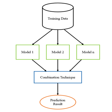Figure 3: General idea of ensemble method

As shown in Figure 3, the major elements of ensemble method are:

1. Training Data: dataset of the problem
2. Ensemble Models: the set of neural network methods used in ensemble
3. Combination Technique: the way to produce final prediction from output of ensemble models

Varying any one of these elements will influence the performance of the ensemble model. It is a challenge to find the best selection to have a final optimal model. The details of each element are explained below.

Training Data

Varying the training data for each model of the ensemble can be done in different ways. The popular one is k-fold cross validation. In the k-fold cross validation, the dataset is divided into k-samples, where each sample is different than the other. A k-models are used for ensemble, where each model uses one sample from a k-samples set.

Bootstrap aggregation, or shortly bagging, is another approach. Here, the dataset is resampled by replacement, and a new dataset is fed into the training model. The composition of each dataset is different, thereby generating different errors from the models. Another approach involves a random selection of data from the dataset.

Training the ensemble models with different samples from the dataset will examine the performance of the model for the different data. It is preferable to have a low correlation in the prediction results of each ensemble members. The predictions of each model are then combined which greater stability and better performance prediction.

Ensemble Models

The performance of any learning algorithm depends on the initial conditions, that is, the selection of hyperparameters to tune algorithm in a way to produce an optimal result. The model can give many results depending on the selection, some that are good, and others that are not. Training more than one algorithm will result in a set of sub-optimal solutions that when averaging them may give an improved estimate.

Each model will produce an error. The model selection should be in a way that results in a low correlation of errors made by each model. To achieve this, it is recommended to tune each model with different capacity and conditions (different number of neurons and layers and different learning rate, etc.).

Combination Techniques

There are three ways of combining model prediction into the ensemble prediction which are:

1. Bagging: Choose different subsamples from the dataset to build multiple models for each sample. The final output is the average of each prediction for all of the sub-models. There are different bagging models such as:
2. Bagged Decision Tree: Performs well with algorithms that have high variance.
3. Random Forest: An extension of Bagged Decision Tree where samples are taken by replacement.
4. Extra Trees: A modification of Bagged Decision Tree where random trees are constructed from samples of the training dataset.
5. Boosting: Build multiple models where each learn to fix the prediction error of the model before it in the chain. The common boosting ensemble models are:
6. AdaBoost: Works by weighing instances in the dataset, so the algorithm can pay less or more attention to their weight while building subsequent models.
7. Stochastic Gradient Boosting: A random subsample of the training data is selected at each iteration and used to fit the base learner.
8. Voting: Build multiple models with some statistics (such as mean) to combine prediction.

A summary of ensemble machine learning algorithms used to enhance performance of models on forecasting problems is shown in Figure 4.

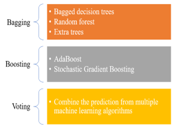Figure 4: Ensemble Machine Learning Algorithms

4.2.  Ensemble Learning Applications

Ensemble learning methods have been applied in different forecasting applications and decision making in various applications [64, 65]. It has been shown in that efficiency of ensemble models is greater than single model in terms of accuracy [66, 67]. A summary of some of those applications are introduced below.

Siwek and Osowski used wavelet transformation and ensemble of neural networks to improve accuracy of prediction of PM10 [66]. The authors applied four neural networks: Multilayer perceptron, Support vector machine for regression, Elman network and radial basis function network. All of them are different and independent.

A randomly selected data samples from the entire dataset is fed to each model, and the final output of each model is fed into another neural network. The results of the proposed model show an improvement in the performance in terms of accuracy.

In the biomedical field, Peimankar and Puthusserypady proposed an ensemble model using recurrent neural networks to detect P-wave in electrocardiogram. The authors used four deep recurrent neural networks. The four networks are trained on the data to extract features, where their output is combined for the final detection of P-waves. The results show a high classification accuracy [67]. Tan, Et al., proposed an ensemble of recurrent neural networks for predicting enhancers, a DNA fragment [68]. In wind forecasting application, Cheng. et al., proposed an ensemble method for probabilistic wind forecasting. The authors used recurrent neural network with different architecture (LSTM, GRU and Dropout layer) for ensemble models, and adaptive neuro fuzzy inference system which were used for combination of final prediction [69]. An adaptive boosting (AdaBoost) combined with Extreme Learning Machine (ELM) for multi-step wind speed forecasting proposed in [70].

Table 3: Analysis of ensemble methods in time-series forecasting applications

Related works	Ensemble method	Combination method	Number of base models	Application domain	Results
Siwek and Osowski [66]	Neural network ensemble	Non-linear mixing	10	Air pollution prediction	Mean Absolute Error (MAE), The Mean Absolute Percentage Error (MAPE), The Root Mean Square Error (RMSE), Correlation Coefficient (R) and Index of Agreement (IA)
Peimankar and Puthusserypady [67]	LSTM ensemble	Dempster-Shafer theory (DST)	4	P-waves detection in ECG recordings	Achieved 98.48% accuracy and 97.22% sensitivity
Tan, Et al. [68]	Bagging	Voting	8	Enhancer classification	achieved sensitivity of 75.5%, specificity of 76%, accuracy of 75.5%, and Matthews Correlation Coefficient (MCC) of 0.51
Cheng. et al. [69]	Hybrid ensemble of wavelet threshold denoising (WTD), RNN and Adaptive Neuro Fuzzy Inference System (ANFIS)	ANFIS	6	Wind speed prediction	(RMSE), (MAE) and normalized mean absolute percentage error (NMAPE)
Peng, et al. [70]	A combination of the improved AdaBoost.RT algorithm with the Extreme Learning Machine (ELM)	Additive of models	5	Wind speed forecasting	RSME, MAE and MASE
Borovkova and Tsiamas [71]	Stacking	Average	12	Intraday stock predictions	AUC
Qi, et al. [72]	Bagging	Voting	8	Chinese Stock Market	accuracy is 58.5%, precision is 58.33%, recall is 73.5%, F1 value is 64.5%, and AUC value is 57.67%
Choi and Lee [73]	LSTM ensemble	Adaptive Weighting	10	Time-series forecasting	(MAE) and (MSE)[

In the stock market prediction, many studies have been proposed based on ensemble methods. Borovkova and Tsiamas proposed an ensemble using LSTM for intraday stock predictions [71]. Qi, et al., used eight LSTM neural network with Bagging method to establish ensemble model for the prediction of Chinese Stock Market [72]. A general time-series forecasting model was proposed in [73] using LSTM ensemble model. The authors used multiple LSTM models where final prediction outputs are combined in a dynamically adjusted way. Table 3 summarize the analysis of previous works.

4.3.  Discussion of related works

Ensemble learning is the method that combines multiple models to enhance prediction accuracy over one model performance. Analysing the challenges of using ensemble method in the time-series applications includes advantages and disadvantages of combination technique used. Table 4 summarize advantages and disadvantages of each ensemble combination method discussed in this paper [74, 75].

Table 4: Advantages and disadvantages of ensemble method

Method	Advantages	Disadvantages
Bagging	–          Used for classification and regression problems –          Performs well in the presence of noise –          Each model works separately	–          Need to perform multiple pass on the dataset –          Dataset size should be known in advance
Boosting	–          Improve power of weak model –          Fast and simple –          Can identify noise	–          Need to perform multiple pass on the dataset –          AdaBoost is sensitive to outliers –          Accuracy is influenced by sufficiency of data
Voting	–          Accuracy increases as number of member increases	–          High computational time

When designing a predictive model for time-series application based on ensemble method, the size affect performance of model. As the number of base models increases, the accuracy improves but will lead to increasing in the computational time and storage space [76]. Determining the optimal number of base models is a research challenge. Some related works proposed the use of pruning ensemble which reduce complexity and enhance performance [77, 78, 79].

In order to increase performance of ensemble model, it is recommended to use different samples for different base models with different features for each model, and to tune each model with different selection of hyperparameters to increase diversity [80].

5. Ensemble Recurrent Neural Network Method

Based on the analysis of previous studies that have been designed as an ensemble model, the framework for ensemble of recurrent neural network for time-series applications can be divided into two main phases: Data Preparation Phase and Ensemble Model Design Phase. The details of each phase are:

1. Data Preparation: Getting the data ready for machine learning algorithm. It is not useful to use real values of data for learning. The data should be consistent, within the same range, and not contain any noise. This includes the following steps:
2. Data Decomposition: Time-series data can be divided into systematic and non-systematic. The systematic data comprises of components from time-series data that are consistent and recurrent. Non-systematic data are components that are not consistent and considered as noise. The systematic components can be defined as follow:
3. Level: The average value of the series data.
4. Trend: Increasing or decreasing of data.
5. Seasonality: Repetitive patterns in the data.

Time-series data can be viewed as a level of components depending on the degree of consistency of the dataset. Splitting the data to components can be useful for better understanding of the problem during time forecasting.

1. Cleaning: Cleaning data from missing and noise values.
2. Normalization: Useful to normalize data to be within the same range, usually between -1 and 1. Two popular choices can be used: minmax scaler and standard scaler.
3. Data Transformation: There are different ways to transform data for processing, which depends on the problem domain. For time-series problem, the data should be re-framed as a supervised machine learning problem. This means that output from previous time step is transformed into an input for the next time step.
4. Data Split: Dividing data into two subsets, training and testing. Usually data is split into 80% training and 20% testing.
5. Features Engineering: This phase includes a processing of data to select most important features that influence the prediction results. In most machine learning applications, feature importance is an essential step which can be performed in numerous ways. For time-forecasting prediction problem, most of the previous works applied mathematical correlation to find a relationship between input and output variables [51, 24, 52, 53, 56]. When there are many features to be entered into the network for training, then finding the correlation between the target output value and these features will reduce complexity of training and enhance performance. The model can then be used with proper input features that can effect on the prediction.

Pearson correlation is the most popular method used to find correlation between two variables.

5. Ensemble Models Selection: This phase contains two main steps:
6. Determining the recurrent neural network models (LSTM, GRU, Bidirectional, etc) which will be used on ensemble design.
7. Hyperparameters Tuning by designing selected algorithms by setting different hyperparameters selection. This means that each algorithm will generate a different error where the correlation between the error values for all algorithms will be low enough to achieve generalization of the model.
8. Combining Models Prediction: The results from each model of ensemble algorithms will be combined using one of the combination ensemble techniques, as described previously, to generate the final prediction of the model.

The overall framework proposed in this paper is presented in Figure 5.

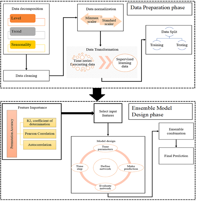Figure 5: ensemble of recurrent neural network framework

6. Conclusions

This paper reviewed several studies that have been applied on recurrent neural network for time-series forecasting applications. The reviewed works give an idea of how to conduct a research for air pollution forecasting using optimization techniques of recurrent neural network and ensemble method. The proposed idea can be formulated on the framework which is divided into two main phases: Data preparation phase and Ensemble model design phase. The Data preparation phase is responsible on cleaning, normalizing and transforming data to a supervised form.

The output of this phase will generate a more consistent data with no noise, duplication and unrelated information. Having consistent training data will affect on the performance by increasing prediction accuracy. Ensemble model design phase includes the choosing of best recurrent neural network design after tuning each model with different parameters, ensemble method type and combination technique. It is recommended to use different subset of samples, different features for each model and tune each model with different parameters to achieve diversity.

The proposed model can be applied in most time-series forecasting applications. This paper focuses on the air pollution forecasting where ensemble method of recurrent neural networks could be suitable for pollution estimation.

Conflict of Interest

The authors declare no conflict of interest.

1.  Lelieveld, J., Evans, J. S., Fnais, M., Giannadaki, D. & Pozzer, A. (2015). “The contribution of outdoor air pollution sources to premature mortality on a global scale”. Nature
2.  WHO Global Ambient Air Quality Database. https://www.who.int/airpollution/data/en/. Accessed:393 2019-08-17
3.  Zheng, Y., Liu, F., Hsieh, H. (2013). “U-Air: when urban air quality inference meets big data”. In: Proceedings of the 19th ACM SIGKDD. International Conference on Knowledge Discovery and Data Mining
4.  Baklanov, A., Mestayer, P.G., Clappier, A., Zilitinkevich, S., Joffre, S., Mahura, A., Nielsen, N.W. (2008). “Towards improving the simulation of meteorological fields in urban areas through updated/advanced surface fluxes description”. Atmospheric Chemistry and Physics
5.  Kim, Y., Fu, J.S., Miller, T.L. (2010). “Improving ozone modeling in complex terrain at a fine grid resolution: Part Ieexamination of analysis nudging and all PBL schemes associated with LSMs in meteorological model”. Atmospheric Environment
6.  Jeong, J.I., Park, R.J., Woo, J., Han, Y., Yi, S. (2011). “Source contributions to carbonaceous aerosol concentrations in Korea”. Atmospheric Environment
7.  Vautard, R., Builtjes, P., Thunis, P., Cuvelier, C., Bedogni, M., Bessagnet, B., Honore, C., Moussiopoulos, N., Pirovano, G., Schaap, M. (2007). “Evaluation and intercomparison of Ozone and PM10 simulations by several chemistry transport models over four European cities within the CityDelta project”. Atmospheric Environment
8.  Stern, R., Builtjes, P., Schaap, M., Timmermans, R., Vautard, R., Hodzic, A., Memmesheimer, M., Feldmann, H., Renner, E., Wolke, R. (2008). “A model intercomparison study focussing on episodes with elevated PM10 concentrations”. Atmospheric Environment
9.  Lee, M.; Brauer, M.; Wong, P.; Tang, R.; Tsui, T. H.; Choi, C.; Chang, W.; Lai, P. C.; Tian, L.;Thach, T. Q.; Allen, R.; Barret, B. (2017). “Land use regression modeling of air pollution in high-density high-rise cities: A case study in Hong Kong”. Science of The Total Environment
10.  Nhung, N. T.; Amini, H.; Schindler, C.; Joss, M. K.; Dien, T. M.; ProbstHensch, N.; Perez, L.; Künzli, N. (2017). “Short-term association between ambient air pollution and pneumonia in children: A systematic review and meta-analysis of time-series and casecrossover studies”. Environmental Pollution
11.  Zafra, C.; Ángel, Y.; Torres, E. (2017). “ARIMA analysis of the effect of land surface coverage on PM10 concentrations in a high-altitude megacity”. Atmospheric Pollution Research
12.  Cannon, A. J.; Lord, E. R. (2008). “Forecasting summertime surface level ozone concentrations in the Lower Fraser Valley of British Columbia: An ensemble neural network approach”. Journal of the Air & Waste Management Association
13.  Zhao, X.; Zhang, R.; Wu, J. L.; Chang, P.C. (2018). “A deep recurrent neural network for air quality classification”. Journal of Information Hiding and Multimedia Signal Processing
14.  A. G. Salman, Y. Heryadi, E. Abdurahman, and W. Suparta, (2018). ‘‘Single layer & multi-layer long short-term memory (LSTM) model with intermediate variables for weather forecasting,’’ Procedia Comput. Sci.
15.  Y. Tsai, Y. Zeng, and Y. Chang, (2018). ‘‘Air pollution forecasting using RNN with LSTM,’’ in Proc. IEEE 16th Int. Conf. Dependable, Autonomic Secure Comput., 16th Int. Conf. Pervasive Intell. Comput., 4th Int. Conf. Big Data Intell. Comput. Cyber Sci. Technol. Congr. (DASC/PiCom/DataCom/CyberSciTech), Athens, Greece
16.  Jae Young Choi and Bumshik Lee, (2018). “Combining LSTM Network Ensemble via Adaptive Weighting for Improved Time Series Forecasting”, Mathematical Problems in Engineering
17.  Yu, S.; Mathur, R.; Schere, K.; Kang, D.; Pleim, J.; Otte, T. (2007). “A detailed evaluation of the Eta-CMAQ forecast model performance for O3, its related precursors, and meteorological parameters during the 2004 ICARTT study”. J. Geophys. Res.
18.  Wang, Y.J.; Zhang, K.M. (2009). “Modeling near-road air quality ssing a computational fluid dynamics model”, CFD-VIT-RIT. Environ. Sci. Technol.
19.  Tong, Z.; Zhang, K.M. (2015). “The near-source impacts of diesel backup generators in urban environments”. Atmos. Environ.
20.  Tong, Z.; Baldauf, R.W.; Isakov, V.; Deshmukh, P.; Zhang, M.K. (2016). “Roadside vegetation barrier designs to mitigate near-road air pollution impacts”. Sci. Total Environ.
21.  Keddem, S.; Barg, F.K.; Glanz, K.; Jackson, T.; Green, S.; George, M. (2015). “Mapping the urban asthma experience: Using qualitative GIS to understand contextual factors affecting asthma control”. Soc. Sci. Med
22.  Chen, L.-J.; Ho, Y.-H.; Lee, H.-C.; Wu, H.-C.; Liu, H.-M.; Hsieh, H.-H.; Huang, Y.-T.; Lung, S.-C.C. (2017). “An Open Framework for Participatory PM2.5 Monitoring in Smart Cities”. IEEE Access
23.  Jiangshe Zhang and Weifu Ding, (2017). “Prediction of Air Pollutants Concentration Based on an Extreme Learning Machine: The Case of Hong Kong”, Environmental Research and Public Health
24.  Xiang Li, Ling Peng, Xiaojing Yao, Shaolong Cui, Yuan Hu, Chengzeng You, Tianhe Chi, (2017). “Long short-term memory neural network for air pollutant concentration predictions: Method development and evaluation”, Environmental Pllution
25.  Li, C., Hsu, N.C., Tsay, S. (2011). “A study on the potential applications of satellite data in air quality monitoring and forecasting”. Atmos. Environ
26.  Box, G.E.P., Jenkins, G.M. (1976). “Time series analysis: forecasting and control”. J. Operational Res. Soc
27.  Nieto, P.G., Combarro, E.F., Del Coz Díaz, J.J., Monta~ nes, E. (2013). “A SVM-based regression model to study the air quality at local scale in Oviedo urban area (Northern Spain): a case study”. Appl. Math. Comput
28.  Hooyberghs, J., Mensink, C., Dumont, G., Fierens, F., Brasseur, O. (2005). “A neural network forecast for daily average PM 10 concentrations in Belgium”. Atmos. Environ
29.  Díaz-Robles, L.A., Ortega, J.C., Fu, J.S., Reed, G.D., Chow, J.C., Watson, J.G., MoncadaHerrera, J.A. (2008). “A hybrid ARIMA and artificial neural networks model to forecast particulate matter in urban areas: the case of Temuco, Chile”. Atmos. Environ
30.  Mishra, D., Goyal, P. (2016). “Neuro-fuzzy approach to forecast NO2 pollutants addressed to air quality dispersion model over Delhi, India”. Aerosol Air Qual. Res
31.  Martha A. Zaidan 1, Lubna Dada, Mansour A. Alghamdi, Hisham Al-Jeelani, Heikki Lihavainen, Antti Hyvärinen and Tareq Hussein, (2019). “Mutual Information Input Selector and Probabilistic Machine Learning Utilisation for Air Pollution Proxies”, Applied Sciences
32.  A. G. Salman, Y. Heryadi, E. Abdurahman, and W. Suparta, (2018). ‘‘Single layer & multi-layer long short-term memory (LSTM) model with intermediate variables for weather forecasting,’’ Procedia Comput. Sci., vol. 135, pp. 89–98
33.  Y. Tsai, Y. Zeng, and Y. Chang, (2018). ‘‘Air pollution forecasting using RNN with LSTM,’’ in Proc. IEEE 16th Int. Conf. Dependable, Autonomic Secure Comput., 16th Int. Conf. Pervasive Intell. Comput., 4th Int. Conf. Big Data Intell. Comput. Cyber Sci. Technol. Congr. (DASC/PiCom/DataCom/CyberSciTech), Athens, Greece, pp. 1074–1079.
34.  Yuelei Xiao and Yang Yin, (2019). “Hybrid LSTM Neural Network for Short-Term Traffic Flow Prediction”, information
35.  E. C. Eze, C.R Chatwin, (2019). “Enhanced Recurrent Neural Network for Short-term Wind Farm Power Output Prediction”, Journal of Applied Science
36.  Olah, C. (2018). “Understanding LSTM Networks”. Available online: http://colah.github.io/posts/2015-08Understanding-LSTMs
37.  Graves, A.; Schmidhuber, J.; Koller, D.; Schuurmans, D.; Bengio, Y.; Bottou, L. (2009). “Offline Handwriting Recognition with Multidimensional Recurrent Neural Networks”. In Advances in Neural Information Processing Systems 21; Curran Associates, Inc.: Dutchess County, NY, USA, pp.545–552.
38.  Yang, Y.; Zhou, J.; Ai, J.; Bin, Y.; Hanjalic, A.; Shen, H.T.; Ji, Y. (2018). “Video Captioning by Adversarial LSTM”. IEEE Trans. Image Process. 27, 5600–5611
39.  Eck, D.; Schmidhuber, J. (2002). “Learning the Long-Term Structure of the Blues”. In Proceedings of the Artificial Neural Networks—ICANN 2002, Madrid, Spain
40. Bengio, Y.; Simard, P.; Frasconi, P. (1994). “Learning long-term dependencies with gradient descent is dificult”. IEEE Trans. Neural Netw. 5, 157–166 Hochreiter, S.; Schmidhuber, J. (1997). “Long short-term memory”. Neural Comput. 9, 1735–1780.
41. Yan, S. “Understanding LSTM and Its Diagrams”. Available online: https://medium.com/mlreview/ understanding-lstm-and-its-diagrams-37e2f46f1714
42.  Cho,K.; Van Merriënboer, B.; Gulcehre, C.; Bahdanau, D.; Bougares, F.; Schwenk, H.; Bengio, Y. (2014). “Learning Phrase Representations using RNN Encoder–Decoder for Statistical Machine Translation”. In Proceedings of the 2014 Conference on Empirical Methods in Natural Language Processing (EMNLP), Doha, Qatar
43.  Chung, J.; Gulcehre, C.; Cho, K.; Bengio, Y. (2014). “Empirical evaluation of gated recurrent neural networks on sequence modelling”. In Proceedings of the NIPS 2014 Workshop on Deep Learning, Montreal, QC,Canada
44.  Schuster, M.; Paliwal, K.K. (1997). “Bidirectional recurrent neural networks”. IEEE Trans. Signal Process, 45, 2673–2681.
45.  Graves, A.; Jaitly, N.; Mohamed, A. (2013). “Hybrid speech recognition with Deep Bidirectional LSTM”. In Proceedings ofthe2013 IEEE Workshop on Automatic Speech Recognition and Understanding, Olomouc, Czech Republic
46.  Saleh Albelwi and Ausif Mahmood. (2017). “A framework for designing the architectures of deep convolutional neural networks”. Entropy
47.  Sean C Smithson, Guang Yang, Warren J Gross, and Brett H Meyer. (2016). “Neural networks designing neural networks: multi-objective hyper-parameter optimization”. In Computer-Aided Design (ICCAD), 2016 IEEE/ACM International Conference on, pages 1–8. IEEE
48.  Nitish Srivastava, Geoffrey Hinton, Alex Krizhevsky, Ilya Sutskever, Ruslan Salakhutdinov, (2014). “Dropout: A Simple Way to Prevent Neural Networks from Overfitting”, Journal of Machine Learning Research 15
49.  Y. Lim, I. Aliyu and C. Lim, (2019). “Air Pollution Matter Prediction Using Recurrent Neural Networks with Sequential Data”, Conference paper, DOI: 10.1145/3325773.3325788
50.  Chiou-Jye Huang and Ping-Huan Kuo, (2018). “A Deep CNN-LSTM Model for Particulate Matter (PM2.5) Forecasting in Smart Cities”, sensors
51.  QING TAO, FANG LIU, YONG LI, AND DENIS SIDOROV, (2019). “Air Pollution Forecasting Using a Deep Learning Model Based on 1D Convnets and Bidirectional GRU”, IEEE Access
52.  Xiaotong Sun, Wei Xu, Hongxun Jiang, (2019). “Spatial-temporal Prediction of Air Quality based on Recurrent Neural Networks”, Proceedings of the 52nd Hawaii International Conference on System Sciences
53.  Athira V, Geetha P, Vinayakumar R, Soman K P, (2018). “DeepAirNet: Applying Recurrent Networks for Air Quality Prediction”, International Conference on Computational Intelligence and Data Science
54.  Thanongsak Xayasouk, Guang Yang, HwaMin Lee, (2019). “Fine Dust Predicting using Recurrent Neural Network with GRU”. International Journal of Innovative Technology and Exploring Engineering (IJITEE)
55.  Brian S. Freeman, Graham Taylor, Bahram Gharabaghi & Jesse Thé, (2018). “Forecasting air quality time series using deep learning”, Journal of the Air & Waste Management Association
56.  K Srinivasa Rao, Dr. G. Lavanya Devi, N. Ramesh, (2019). “Air Quality Prediction in Visakhapatnam with LSTM based Recurrent Neural Networks”, I.J. Intelligent Systems and Applications
57.  Xiaosong Zhao, Rui Zhang, Jheng-Long Wu and Pei-Chann Chang, (2018). “A Deep Recurrent Neural Network for Air Quality Classification”, Journal of Information Hiding and Multimedia Signal Processing
58.  Hamed Karimian, Qi Li2, Chunlin Wu, Yanlin Qi, Yuqin Mo, Gong Chen, Xianfeng Zhang and Sonali Sachdeva, (2019). “Evaluation of Different Machine Learning Approaches to Forecasting PM2.5 Mass Concentrations”, Aerosol and Air Quality Research
59.  Widya Mas Septiawan and Sukmawati Nur Endah, (2018). “Suitable Recurrent Neural Network for Air Quality Prediction With Backpropagation Through Time”, 2nd International Conference on Informatics and Computational Sciences
60.  Zhou and Jiang, NeC4.5: (2004). “Neural Ensemble Based C4.5”. IEEE Transactions on Knowledge and Data Engineering, vol. 16, no. 6, pp. 770-773
61.  Zhou Z. H., and Tang, W. (2003). “Selective Ensemble of Decision Trees”. Internationl workshop on: Rough Sets, Fuzzy Sets, Data Mining, and Granular-soft, pp.476-483
62.  Kok Keng Tan, Nguyen Quoc Khanh Le , Hui-Yuan Yeh, and Matthew Chin Heng Chua, (2019). “Ensemble of Deep Recurrent Neural Networks for Identifying Enhancers via Dinucleotide Physicochemical Properties”, Cells
63.  A.Peimankar,S.J.Weddell,T.Jalal,andA.C.Lapthorn, “Evolutionary multi-objective fault diagnosis of power transformers,” Swarm and Evolutionary Computation, 2017. vol. 36, pp. 62–75.
64.  Polikar, (2006). “Ensemble based systems in decision making,” IEEE Circuits and systems magazine, vol.6, no.3, pp. 21–45
65.  A.Peimankar, S.J. Weddell, T.Jalal, and A .C. Lapthorn, (2018). “Multi-objective ensemble forecasting with an application to power transformers,” Applied Soft Computing, vol. 68, pp. 233–248
66.  Hochreiter and J. Schmidhuber, (1997). “Long short-term memory,” Neural Computation, vol. 9, no. 8, pp. 1735– 1780
67.  Siwek and S.Osowski, (2012). “Improving the accuracy of prediction pf PM10 pollution by the wavelet transformation and an ensemble of neural predictors”, Engineering Applications of Artificial Intelligence
68.  Abdolrahman Peimankar and Sadasivan Puthusserypady, (2019). “AN ENSEMBLE OF DEEP RECURRENT NEURAL NETWORKS FOR P-WAVED ETECTION IN ELECTROCARDIOGRAM”, ICASSP
69.  Kok Keng Tan, Nguyen Quoc Khanh Le, Hui-Yuan Yeh and Matthew Chin Heng Chua, (2019). “Ensemble of Deep Recurrent Neural Networks for Identifying Enhancers via Dinucleotide Physicochemical Properties”, Cells
70.  Lilin Cheng, Haixiang Zang , Tao Ding , Rong Sun , (2018). Miaomiao Wang, Zhinong Wei and Guoqiang Sun, “Ensemble Recurrent Neural Network Based Probabilistic Wind Speed Forecasting Approach”, Energies
71.  Peng, T.; Zhou, J.Z.; Zhang, C.; Zheng, Y. (2017). “Multi-step ahead wind speed forecasting using a hybrid model based on two-stage decomposition technique and AdaBoost-extreme learning machine”. Energy Convers. Manag
72.  Svetlana Borovkova and Ioannis Tsiamas, (2019). “An ensemble of LSTM neural networks for high-frequency stock market classification”, Wiley
73.  Xie Qi, Cheng Gengguo, Xu Xu and Zhao Zixuan, (2018). “Research Based on Stock Predicting Model of Neural Networks Ensemble Learning”, MATEC Web of Conferences 232, 02029
74.  Jae Young Choi and Bumshik Lee, (2018). “Combining LSTM Network Ensemble via Adaptive Weighting for Improved Time Series Forecasting”, Mathematical Problems in Engineering de Souza, E. N., & Matwin, S. (2013). “Improvements to Boosting with Data Streams Advances in Artificial Intelligence” (pp. 248-255): Springer
75.  Oza, N. (2001). Online Ensemble Learning. (PhD), University of California, Berkeley
76.  Antonino A. Feitosa Neto, Anne M. P. Canuto and Teresa B Ludermir, (2013). “Using Good and Bad Diversity Measures in the design of Ensemble Systems: A Genetic Algorithm Approach”, IEEE Congress on Evolutionary Computation, pp. 789 – 796. IEEE
77.  Lacoste, A., Larochelle, H., Laviolette, F., & Marchand, M. (2014). “Sequential Model-Based Ensemble Optimization” arXiv preprint arXiv:1402.0796
78.  E. Banfield, L. O. Hall, K. W. Bowyer and W. P. Kegelmeyer. (2002). “Ensemble Diversity Measures and Their Application to Thinning”, Information Fusion, vol. 6, no. 1, pp. 49-62, Elsevier B.V
79.  Sylvester, J., Chawla, N. (2006). “Evolutionary Ensemble Creation and Thinning”, In: IJCNN 06 International Joint Conference on Neural Networks, pp. 51485155, IEEE.
80.  Wang, S., & Yao, X. (2013). “Relationships Between Diversity of Classification Ensembles and Single-Class Performance Measures”, Knowledge and Data Engineering, IEEE Transactions on, vol. 25, No. 1, pp. 206219. IEEE.

(Click Here)

(Click Here)