1. Introduction

The Wind energy provide a vast energy contribution to the modern world energy requirements. Recently its development made a huge impact to the world energy needs. Wind energy has a long history for more than 130 years [1]. In the early age of the wind industry, windmills were used to pump water for farms. Nowadays larger scale wind turbines can produce up to 10MW and Small wind turbines can produce less than 100 kilowatts. However, management of the wind energy sources has been always challenging as it has a considerable effect on different aspects of the power system such as the power quality [2], power harmonics and inter-harmonics [3], power line communications [4], etc. In this regard, research topics regarding how to obtain a maximum power output for high speed wind input without destroying the small-scaled wind turbine system can be considered as one of the important research areas of the wind energy. Because in high speed wind conditions the turbines output could be overloaded and could destroy the small-scaled wind turbine due to low inertia momentum. Therefore, in such wind condition, the wind operation must be stopped to avoid being damage to the small scaled wind turbine.

In this research, our work is about how to operate the wind turbine in such storm condition and how to generate the electricity without damaging the turbine. In the simulation results we have shown that it is possible to use eddy current magnetic brake system on the proposed method for the stall control. Wind turbine brake system plays an important role when there is storm condition. Most of the modern wind turbines use the friction brakes to control the rotation of the rotor of the wind turbine [5]. The brake pads are the important part to slower or stop the rotation of the rotor in strong wind situation. Therefore, these brake pads should be made for long term use. But still the modern wind turbine brakes can be used for few years, after that either it should be repaired or replaced by a new brake pad. Therefore, our aim is to introduce this magnetic brake system to replace the current friction brake system. The main specialty of this magnetic brake is there is no mechanical contact with the rotor for controlling the speed of the turbine. Therefore, this eddy current brake system is an alternative method to the conventional friction-based brake system [6]. Also, magnetic brake system required less maintenance than the conventional brake system [7].

In this paper, at first, we explain about small-scaled wind turbine blade which is destroyed due to experimental tension test that equivalent to centrifugal force due to over rotation of the blade. Afterwards the application of the magnetic brake and the eddy current brake were introduced. Later the mathematical modeling of the system and simulation results were explained.

2. Analogical experiment of blade destruction

Wind turbine blades are often destroyed by strong winds. The reason is due to the centrifugal force on the blades triggers into over-rotation by strong winds. In order to realize a tensile force equivalent to the centrifugal force until the blade destroys, the blade was subject to a tensile test. Figure 1 shows the test status of the broken wind turbine blade. In otherwords, this analogical experiment is done in order to obtain the safety margin of the blade. This experiment stands for loading force (i.e. equivalent to centrifugal force) to the blade until it breaks out. Through this experiment we can calculate the force that may cause destruction of the blade. Once the destructive force is obtained then we can re-calculate the maximum allowed angular velocity. The material of the blade is made by FRP (Fiber Reinforced Plastic). Figure 2 shows the experimental results of tension test of the blade. In this figure the horizontal axis stands for the displacement of the blade against the axis of the blade. Then vertical axis shows the tension force to the blade. Figure 2 was obtained using Microsoft Excel software. In this experiment, when the tensioned force reach to approximately 27 kN, at that point the blade is destroyed. So, in order to avoid such destruction, we have to concern safety margin. As it is obvious in Figure 2, tensioned force is linear with respect to displacement up to 6 mm. However, after 6mm the characteristics of the blade becomes non-linear against to force. Concerning safety margin and non-linearity of curve, we set the maximum allowed force to 4.5kN.

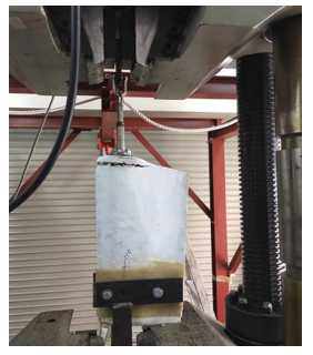Figure 1. Broken wind turbine blade

Equation (1) shows the relation between tensioned force that is equivalent to centrifugal force and angular velocity as well the parameter and value are shown in table 1 below this equation.  stands for allowable maximum force, m is the weight and r is the length of blade.

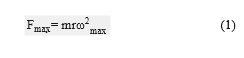Table 1: Specification of the blade

Parameter	Value	Unit
	4.5	kN
	4.5	kg
	1	m
(without margin)	31.622	rad/s

According to equation (1) and table 1, the allowable maximum angular velocity   is 31.622 rad/s (point A in the Figure 2). which is 4.5kN. We did not set the maximum angular velocity to the obtained value since safety margin is taken. Therefore, we put a secondary safety margin value as 29 rad/s (point B in the Figure 2) and primary safety margin value as 25 rad/s (point C). By doing so, we can obtain low penetration value 3.8kN for 29rad/s and 1kN for 25rad/s which is less than 4.5kN. From point A to point D can be considered as the blade destruction area. After point D the blade was broken. Hence, we set the as follows,25rad/s.

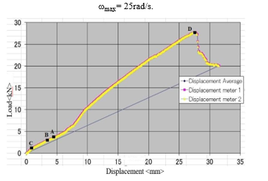Figure 2. Blade destruction chart

3. Mechanism of eddy current brake

3.1.  Eddy current theory

 Some specific theories are related to the eddy current theory, such as the Faraday law of induction, the Lenz law and Fleming’s right hand rule. Eddy current theory-based instruments are currently applied on many areas modern day. Some examples include bomb detectors and Electric meter for residence, among others.

Faraday law of induction states that a magnetic field can produce a current in a closed circuit when the magnetic flux linking to the circuit is changing [8]. Equation (2) introduces the mathematical expression of the Faraday law of induction,

where, ε and Φ stands for electromotive force and magnetic flux, respectively.

Assuming this magnetic flux induced on a copper plate and its resistor is R_C and I is the induced eddy current on a copper plate. We can obtain the mathematical expression as (3), According to ohm’s law,

From (2) and (3) we can obtain the eddy current as the following equation indicates.

Therefore, it can be stated that induced eddy current can be calculated using (4).

3.2.  Lenz law

Lenz law states that the direction of an induced electromagnetic force (e.m.f) is always such that it tends to set up a current opposing the motion or the change of flux responsible for inducing that e.m.f [9]. Eddy currents are the loops of currents which are induced due to the moving of a non-ferromagnetic conductor and a magnetic field according to the Faraday’s law of induction as the equation above highlights. The path of the eddy current induced in the non-ferromagnetic material shaped in the form of a loop and it build up a magnetic field opposite to that of magnet [10]. The blue lines in the Figure 3 display the eddy currents induced on the conductor plate. The magnitude of the eddy current induced in the conductor is proportional to the size of the magnetic field. Also, the rotating copper plate which is attached to the rotor will exert a drag force from the permanent magnet. This drag force will operate as the brake force to control the angular velocity of the small scaled wind turbine. The reason for using the copper plate is that it’s a non-ferromagnetic material. For ferromagnetic materials the eddy current will not be induced.  Each time when the copper plate rotates the magnetic flux on the copper plate is changing. As a result of magnetic flux change the braking force will create due to the interaction of the eddy current on the plate and the magnetic field. Therefore, the magnet exerts a drag force on the copper plate. As a result of this, the rotation of the angular velocity of the copper plate decreases.

Nowadays electromagnetic brake systems are used widely such as in industrial applications, gym appliances, rollercoasters, recreation equipment’s and maglev trains among others. This magnetic brake system is considered as a very efficient brake system because of its non-contact braking operation [11]. The advantage of this braking system is that, when the force become stronger, the magnetic force creates a stronger force against the system, relatively. Figure 3 shows how eddy current brake works. Only one section of the magnets was shown to describe the illustration more precisely. However, in the brake system incorporated multiple magnets to produce a strong braking force on the braking plate.

Figure 4 displays the breaking plate with induced eddy current. B1 and B2 are the induced magnetic field on the copper plate from the magnet.

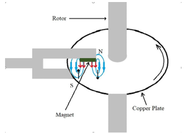Figure 3. Cross section of the brake

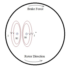Figure 4. Braking plate

Mathematical expression for B is in (5). Here B denotes magnetic flux density and magnetic intensity denotes by H.  represent the permeability of the atmosphere.

The brake force is created as a result of the induced eddy current according to the Fleming’s left-hand rule. While the rotor rotates counterclockwise the braking force will occur in clockwise direction.

4. Conventional method and proposed method and its application

Nowadays the conventional wind turbines use different types of control methods to get an efficient, stable and long-term durability power. Pitch control [12,13], yaw control, friction [14-16] control is popular control method are being used. In the friction control method, the brake pads are being used to control the angular velocity of the rotor. However, such brakes cannot be used long-term, since they need to be repaired or replaced if the brake pads were broken. Our proposed brake system, on the other hand, utilizes a magnetic eddy current brake system which controls the angular velocity in a non-contact manner with the rotor. In spite of the friction brake system that has the contact with the rotor, our proposed method is contactless. Hence, it is adequate for long-term usage, rather than the time span offered by the conventional one.

The arrangement of magnets is displayed in Figure 5 in which the braking torque occurs in the opposite direction of the disk rotation.

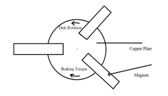Figure 5. Cross section of the brake

When the small-scaled wind turbine angular velocity increases the copper plate angular velocity will increase simultaneously because the plate is attached to the rotor. When copper plate velocity increases the drag force on the plate from the induced eddy current also will be increased. Therefore, the angular velocity of the turbine will be controlled.

4.1.  The structure of proposed brake system

In order to implement the eddy current contact less brake system, we have designed the following system shown in Figure 6. The principle is based on the eddy current occurrence that requires non-ferromagnetic low resistor material is implemented by the cooper plate and magnetic flux is set in the arm as it is shown in Figure 5. The principle of brake system is that when the angular velocity exceeds 25rad/s, the two magnets will be turned in between the copper plates in parallel using the arm that controlled by servo motor. As a result of this matter, due to rotation of plate and changing magnetics flux the emf is induced and eddy current will flow. Consequently, angular velocity of rotor will decrease due to the induced magnetic brake force. Hence, the excessive angular velocity will be restricted to the referenced value. Here, microcontroller has the controller role in the brake system. It measured the angular velocity and control the movement of arm by servo motor. By assumption of following prototype system, we construct the flow diagram of the system in next section.

4.2.  Flow diagram of the system

After the small-scaled wind turbine received the input wind, the flow will divide into mechanical power ( ) and power captured from wind ( ). Then the subtraction of power captured from wind and mechanical power can obtain electrical power ( ). Afterward  will go through 3 φ power generator ( ). Then the power received from the AC generator will distributes to AC/DC converter which includes rectifier and low-pass filter. At this stage the alternate current will convert to the direct current and it will charge the batteries for the purpose of supplying electricity to the DC green-house system. The load is variable. This process is displayed in the Figure 7.

When the measurement system receives the angular velocity  of the small-scaled wind turbine the measurement system will send the measured angular velocity  to the system controller. Afterwards the system controller will obtain the  by calculating the difference between the reference value of angular velocity  and . Then, the system controller will turn on the servo motor to rotate the magnet closer to the braking plates. At this point, the magnetic brake force  will reduce the rotation of the brake plate as a result of the induced eddy current on the copper plate. This process was illustrated in Figure 8. In the next section mathematical modeling of entire system is described in detail.

4.3.  Mathematical modeling

In this section the entire dynamics model of system is introduced. The system consists of small-scaled wind turbine, mechanical shaft, 3φ generator, DC converter and the DC bus in order. The DC bus is providing power to the loads at the end. The pattern of loads is shown in later section.

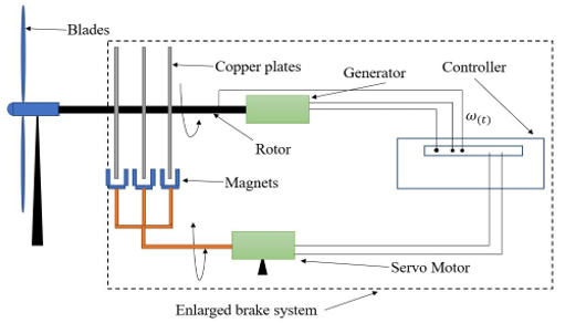Figure 6. Proposed brake system

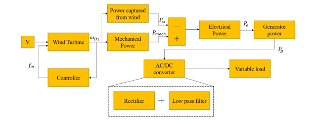Figure 7. Flow diagram of the entire system

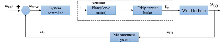Figure 8. Control system block diagram of the proposed system

Table 2: Parameters

Symbol	Name
	Inertia moment of the blade
	Angular Velocity
	Density of atmosphere
	Area swept by blade
	Length of blade
	Speed of wind
	Axis friction factor
	Permeability
	Magnitude of the magnetic field of the magnet
	Magnitude of the magnetic field of the copper plate
	Distance between copper plate and magnet
	Decision functional adjustment
	Reference value of angular velocity
	Measured angular velocity
	Eddy Current
	Power coefficient
	Torque coefficient
	Generator power coefficient
	Rectifier efficiency of DC converter

At first, we introduce the dynamics of the conventional model of small-scale wind turbine and afterwards the dynamics of the proposed method will be shown. The table 2 shows the parameters identification of the whole system. Additionally, the power efficiency of 3 φ generator and DC converter is considered as they are connected to the turbine shaft directly without coupling any gear.

The conventional dynamics of equation (6) represents the dynamics of the conventional small-scaled wind turbine system

In order to show the stability of the system we apply the Laplace transform and made two assumptions to linearize the system

Assumption 1;   is a constant value,

Assumption 2;   = 0.

Since velocity is constant the Laplace transform of the input term can be considered as .

Here, s is the Laplace operator

The Laplace transform of angular velocity and its derivative can be obtain by following transformation rules

Therefore, the Laplace transform of equation (6) is (7)

Through equation (7) we obtain the transfer function of conventional method shown in (8).

For (8) the bode plot is shown in Figure 9 to describe that how angular velocity responds to wind velocity that may contains various frequency components.

The parameter of transfer function is set to as following: = 0.2; = 12;

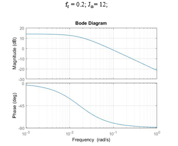Figure 9. Bode diagram of transfer function of (8)

As it can be seen in Figure 9, the gain for low frequency components the output of transfer function will include up to 15 dB. This means that if there is a constant wind velocity (rated velocity) penetrates the turbine, the angular velocity increases rapidly. However, the natural wind velocity spectrum varies from low to high frequencies. As it is clear, in high frequency domain the gain is decreasing drastically. Therefore, the analysis of wind velocity spectrum [17] becomes significant that how affect the turbine rotation behavior. However, in this study we are not go through this.

Next for the stability analysis, from the transfer function we can obtain the pole of conventional method that the denominator of equation (8) is set to be 0. Hence, we have as following:

The system is stable, since the pole is negative. So, we can conclude that the small-scaled wind turbine system has a stable behavior. The proposed method is shown by applying with combination of the eddy current and decision function.

The equation below expresses the proposed torque equation.

The torque equation is shown in Figure 10.

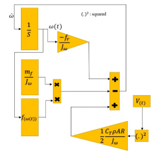Figure 10. Flow of the torque equation

As it is clear in the above equation, conventional method of break system to restrict the angular velocity has done by  which the technique was to varying the friction by brake pad. However, in this study since the  term is proposed as contactless break method, the is considered as the friction of shaft coupled to the generator which can be assumed to be a constant value. Therefore, for the sake of contactless purpose the magnets are utilized in order to magnetize the copper plate and as results the eddy current will flow. The torque earned from term fm is single set permanent magnetic brake torque on the rotor which is

Where, d is the distance from copper to each magnet and  and  stands for magnitude of the magnetic field.

For the sake of stronger torque creation from magnetization, in this study we set 3 sets of permanent magnetic brake in parallel as described in Figure 5, the above equation becomes as follows

Furthermore, equation (12) represents the decision function [18-19].

The decision function acts as a switch to brake system to decide at what moment the exceeds . Therefore, whenever, angular velocity exceeds the reference value it will be activated. However, the performance of decision function depends on the coefficient α_adj  which is analyzed in the later section.

Next ,T_B  is the torque of the blade which can be written as below equation.

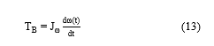Where,  is the inertia moment of the blade.

Finally, T_axis represents the axis friction torque as described as follows

Where,  is axis friction factor.

It is notable that in conventional brake system this term was controlled to regulate and restrict the angular velocity [20]. However, we are not going through it in this paper.

The application of this study is to install 3 φ generator and rectifies its output to provide a DC power supply to the loads.  Load considered to be DC-Green house that will describe the details in later section. The schematic of rectification and smoothing of its output, in other words the conventional DC converter consists of 6 diodes, capacitor and resistor which these two elements are used as the low-pass filter to smoothen the rectified output waves. Figure 11 represents a schematic of the generator which considered to be 3 φ power supply, full wave rectifier and low pass filter and a battery parallel with loads.

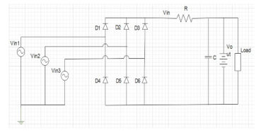Figure 11 Three phase voltage circuit diagram with rectifier and low pass filter.

Equation (15) shows the low pass filter dynamics.

From (15) we can obtain the transfer function of low pass filter shown in following equation (16),

Where, s is Laplace operator.

As it can be seen it is significant to choose the R and C value to obtain a stable output to the loads. However, in this study, we are not going to the detail of designing the low-pass filter.

Now let us consider the power dynamics in order to obtain the anticipated generated electrical power from generator. According to the following equation the subtraction of   by is equivalent to . In other words, mathematical expression is as follows

Since  is obtained by wind turbine characteristic formula, P_e can be anticipated by simple manipulation of above equation.

As mentioned previously, in this study since the efficiency is considered we define an output power efficiency of a 3φ AC generator and its rectification since the load is DC bus.

The output power of the 3φ AC generator displayed in (19).

Here,  is the power coefficient of the generator and  is the electrical power received to the generator.

Further, equation (20) shows the converted DC power.

where,  represents the efficiency of rectifier of DC converter.

As considering the power stability analysis, it is significant that the produced power from wind turbine has adequate capacity of power in order to provide power to the loads. Therefore, the final stage of power conversion that is P_DC, this should satisfy the power to the loads constantly and globally in time domain which includes the transient and steady response.

Suppose that we have a function such as following (21)

which Γ(.,.) stands for remnant function. The remnant function is composed of remnant power normalized by final stage power output that is DC converter output.  Here, if and only if Γ is Semi Positive-definite function then the power supply is globally stable. The Below equation is used to verify the power supply stability.

Once the above equation is satisfied, then the required capacity is adequate for entire system. Besides, for above equation, in any situation  is satisfied so that the load’s installation percentage can be determined. The satisfactory analysis and evaluation is done in later section as simulation.

4.4.  Extension of the proposed method

From now on we will explain the extension of the proposed method which is about adding  and  as variables into the system. In equation (23) l stands for tip speed ratio which is equal to the linear velocity of the wind turbine blade divided by the wind velocity.  is the angular velocity of the blade and R is the radius of the blade [21].

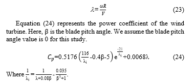In this research pitch angle is assumed to be 0 constantly. Therefore,

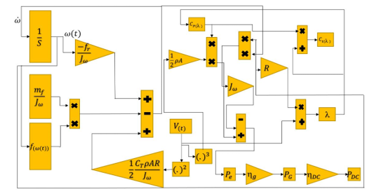Figure 12. Expanded block diagram including  and

Equation (25) displays the torque coefficient

The extended flow diagram of the [22] article is displayed in Figure 12. Note that   and  represent the mathematical operation as squared and cubed of input, respectively.

4.5.  Analysis of decision function behavior

The decision function has an important role to do as regulation of angular velocity while it is operating. When angular velocity is greater than the reference value the decision function value will be greater than 0.5. Then the eddy current brake system will activate to reduce the angular velocity of the rotor.

For behavior analysis of decision function, let’s give an artificial set of angular velocity that is ω = 2×t which t stands for time as shown in Figure 13. We used MATLAB/Simulink software to plot the following figures shows in this section.

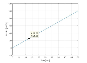Figure 13. Input wind

For performance analysis of decision function  is a critical coefficient. Therefore, we applied different  values such as 0.1, 0.5, 1, 10, 200 to observe the output behavior of decision function. The triggered angular velocity value is set to be 25 rad/s.  For these different  values, the behavior of the decision function with respect to time is shown in Figure 14. For high values of  such as 200 the decision function value is almost 1 at approximately 12 seconds which also can be seen in Figure 13 that at 12 sec angular velocity reaches 25 rad/s. According to Figure 15, when the   is 0.1 the decision function’s output has lower value comparing to the other  values that are greater than unity. The decision function has a lower value in the beginning means that the brake system has already started to work when the angular velocity is below 25rad/s as shown in Figure 15. When the decision function output value is at 0.5 the brake system is triggered. When the  increases the decision function value is converging to 1 for brake mode. That means the system must use a higher  value in order to get an efficient brake control system. According to Figure 15 the highest  value is 200. As it is clear in Figure 15, the area of non-braking mode except α_adj = 200 line (ideal mode) is shown in the gray color mesh and other area is for the braking mode.

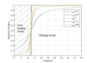Figure 14. Performance of decision function against time

However, in reality it is hard to realize a system with  200 due to microcontroller process time and may not have enough capability to calculate speedily. Therefore, some internal delay may occur in the system and stability and performance analysis should be done for system including time delay element [23-25]. However, in this study, since we focus on behavior of brake system performance, instead of analyzing the delay system we set the     to an acceptable value. Hence, we applied the  as 10 to which has adequate transient response according to Figure 14 and at the same time is considered to be a reasonable value for implementation in actual case.

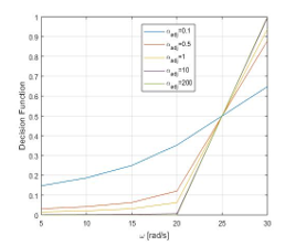Figure 15. Decision function against angular velocity

5. Simulation and Results

In this section, first, we built the mathematical model of the control system then we simulated it in the MATLAB/Simulink based environment. At first we simulate the angular velocity response for different mean velocities from 10 to 30 m/s. Next we set two patterns of input wind velocity and observe the angular velocity behavior. One set is a regular rising and declining wind velocity (pattern No.1) and the other one is a random one (pattern No.2) which are shown in results. Additionally, for each pattern, in order to observe the decision function performance, we have shown the offsets between the ω_ref and ω_steady with respect to = 6 to 200. The offset stands for the subtraction of reference angular velocity by steady response which concerns system performances. Eventually, for both patterns, to observe the power provision stability evaluation function is shown with regard to time response.

5.1.  Simulation conditions

In this simulation, power coefficient and torque coefficients are considered as variables. Previously in [1] power coefficient and torque coefficient were constants. Simulation time for this research is 1000s. Sampling time is 0.1s. The load as shown in Figure 16 is applied to entire simulation. The input load behavior changes depending on various conditions in DC-green house such as weather, temperature, light condition. In the greenhouse the power consumption is varying through day and night time. Specially in night time the power consumption would be higher since many devices are in operation. Such as the LED lights which exposes light to products, microcontrollers and sensors. Therefore, we created the load that applies in real case to verify the proposed system that while restriction of angular velocity weather it is possible to provide an adequate power to the loads or not. However, for the sake of simplicity for analysis as it is expressed duration time is set to 1000 s.

Table 3 displays the parameters values with the SI units

Table 3: Values of the Parameters

Symbol	Value	Unit
	12	kg.
	Variable
	1.225	kg.
	3.14
	1.5	m
	Variable
	0.2
	4π
	62.5*	A.m
	0.1*	A.m
	0.05	m
	10
	25
	0.9
	0.9

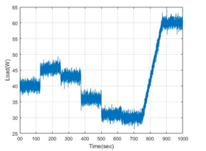 Figure 16. Pattern of the load

5.2.  Results

From now on, Figure 17 to Figure 21 displays the angular velocity behavior for different input average velocities of 10, 15, 20, 25 and 30 m/s in order with controller decision function coefficient is set to α_adj = 10 and the stall angular velocity or the referenced one is considered to be 25 rad/s as it has been chosen in section 2.

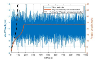Figure 17. Stall control chart for average wind 10m/s

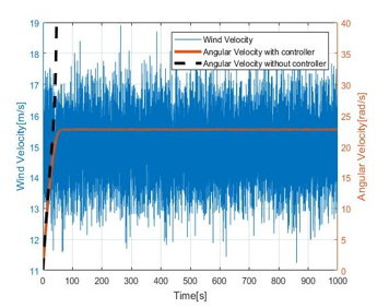Figure 18. Stall control chart for average wind 15m/s

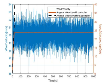Figure 19. Stall control chart for average wind 20m/s

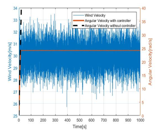Figure 20. Stall control chart for average wind 25m/s

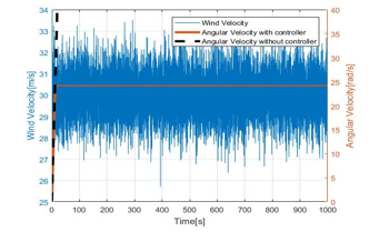Figure 21. Stall control chart for average wind 30 m/s

By analyzing the Figure 17 to Figure 21 it is obvious that the magnetic brake system restricts the angular velocity up to 25 rad/s for average wind velocities of 10m/s to 30m/s. However, without controlling it will diverge and system becomes unstable. Moreover, the transient response of decision function seems to be adequate. Therefore, we can conclude that α_adj = 10 has a stable behavior and acceptable performance. Following Figure 22 summarize the angular velocity behavior when the input wind velocity changes from 10m/s to 30m/s.

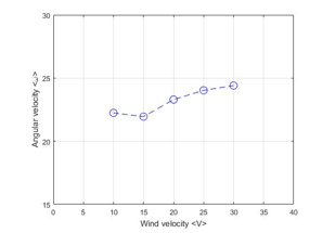 Figure 22. Wind velocity from 10m/s to 30m/s against angular velocity

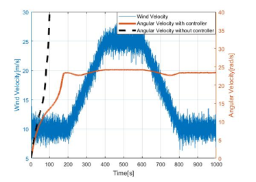Figure 23. Angular velocity behavior for wind velocity pattern No. 1

Figure 23 and 24 explain how the brake system works with and without the proposed control. Angular velocity without the brake control is displayed using the broken line which is diverging on the Y-axis for both wind patterns. The maximum average wind velocity in this simulation is 25m/s and the minimum value is 5m/s. Patterns of input velocity have been created artificially.

As it is shown in above figure, the behavior of angular velocity with proposed controller against the input wind velocity pattern No.1 has a stable attitude with respect to time. As well, it is visible that the angular velocity is controlled up to 25rad/s even during high wind penetration conditions which is during 400 to 600 sec.

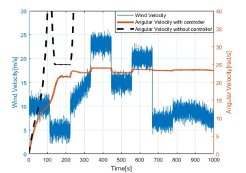Figure 24. Angular velocity behavior for wind velocity pattern No. 2

In Figure 24, it is clear that even though angular velocity with proposed controller fluctuates but it has stable response and have been suppressed up to 25 rad/s and cease the excessive rotation. The arise of fluctuation of angular velocity is due to the wind pattern that have been penetrated to the wind turbine. Therefore, the angular velocity behavior should be enhanced for such sudden changes of wind velocity. However, for now it satisfies the requirement. Therefore, mechanical point of view, we can conclude that the angular velocity can be sustained to a desired or referenced value by proposed method.

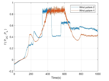Figure 25. Time response of evaluation function for wind pattern 1 and 2

Next the power provision is evaluated by evaluation function which has been defined previously. Following Figure 25 is shown the evaluation function for the wind velocity pattern No. 1 and 2, respectively.

As it is obvious, except the transient duration, equation (21) is satisfied. Hence, the proposed controller can also provide an adequate power supply to loads and restricts the angular velocity.  Also, the power output contains the remnant quantity of power particularly during high wind penetration that means it can be stored to power bank or charges the peripheral batteries.

Finally, in order to ensure the decision function performance that is part of controller the offsets of referenced angular velocity and steady value of angular velocity with controller has been plotted with respect to α_adj in Figure 26.

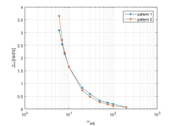Figure 26. Offset for average wind velocity 20m/s

As it is clear in above figure, if the  < 10, then the corresponding offset increase. On the other side,  if   > 10, then the corresponding offset would decrease. This means for higher value of factor, performance of the system improves since the offset decreases. However, as have been discussing, it is fairly hard to set   to high value due to microcontroller processor capability for realization. Therefore,   can be set to 10 according to the above since it is not too high value and at the same time it has sufficient performances.

6. Conclusion

In this paper, we have simulated an eddy current magnetic brake system for the small-scaled wind turbines. In strong wind condition, several types of control methods utilized to get the desired electricity output for small-scaled wind turbines. But still the modern wind turbines unable to get a stable generated electricity output when there is a storm condition. In storm condition, most of the wind turbines stop their operation to protect the turbine and it’s all components. As we have seen from the simulation results it is possible to conclude that using the eddy current brake system, we can limit the angular velocity below 25rad/s when there is storm condition and satisfies the power provision to the loads, simultaneously. Since there is no mechanical connection with the rotor and the brake system, we believe it may be able to use for much longer time than the conventional friction brake system. Thus, for future works, we will apply the Lyapunov function for the stability analysis. Moreover, in this paper the trigger of angular velocity is set based on physical destructive value. However, maximum power point should also be considered for enhancing the efficiency. Therefore, we will use the maximum Power Point Tracking Method (MPPT) to get a maximum power output form objected wind turbine. Additionally, pitch controlling method is a very useful method to control the wind turbine operation. Since we haven’t applied this method to the proposed system in this paper, we will apply pitch control method as future work for this system. Finally, the integration of pitch angle control and proposed eddy current brake system will be implemented.

Conflict of Interest

The authors declare no conflict of interest.

1.  J.F Manwell, J.G. Mcgowan, A.L. Rogers, Wind Energy Explained, John Wiley and Sons, 2009.
2.  E. Santos, M. Khosravy, M.A. Lima, A.S. Cerqueira, CA Duque, “ESPRIT associated with filter bank for power-line harmonics, sub-harmonics and inter-harmonics parameters estimation”. INT. J. ELEC. POWER, 118, p.105731, 2020. https://doi.org/10.1016/j.ijepes.2019.105731
3.  E. Santos, M. Khosravy, M.A. Lima, A.S. Cerqueira, C.A Duque, and A. Yona, “High accuracy power quality evaluation under a colored noisy condition by filter bank ESPRIT” Electronics, 8(11), p.1259, 2019. https://doi.org/10.3390/electronics8111259
4.  A.A. Picorone, T.R. de Oliveira, R. Sampaio-Neto, M. Khosravy, M.V. Ribeiro, “Channel characterization of low voltage electric power distribution networks for PLC applications based on measurement campaign”, INT. J. ELEC. POWER., 116, p.105554. 2020. https://doi.org/10.1016/j.ijepes.2019.105554
5.  Y.B. Lee, G.C. Lee, J.D. Yang, J.W. Park, D.C. Baek, “Failure analysis of a hydraulic power system in the wind turbine” ENG. FAIL. ANAL. 107, 104218, 2020. https://doi.org/10.1016/j.engfailanal.2019.104218
6.  R. Yazdanpanah, M. Mirsalim., “Hybrid electromagnetic brakes: design and performance evaluation” IEEE T. ENERGY CONVER., 30(1), 60-69, 2015. https://doi.org/10.1109/TEC.2014.2333777
7. H. Sodano, J.S. Bae, “Eddy current damping in structures” The Shock and Vibration Digest., 36(6), 469-478, 2004. https://doi.org/10.1177/0583102404048517
8. J. D. Kraus, K. R. Carver, Electromagnetics, 2nd ed. McGraw Hill, 1973.
9. John Bird, Electrical circuit theory and technology. Third edition, Newnes, 2007
10. M. O. Gulbahce, D.A. Kocabas, I Habir, “Finite element analysis of a small power eddy current brake” Proceedings of 15th International Conference MECHATRONIKA, Prague, Czech Republic, 2013.
11.  K.J. Lee, K. Park, “Optimal robust control of a contactless brake system using an eddy current” Mechatronics, 9(6), 615–631, 1999. https://doi.org/10.1016/S0957-4158(99)00008-2
12.  F. Asharif, S. Tamaki, T. Nagado, T. Nagata M.R. Asharif, “Analysis of non-linear adaptive friction and pitch angle control of small-scaled wind turbine system,” Future Generation Information Technology FGIT 2011, Control and Automation CA, Springer-Verlag, Lecture Note: Communication in Computer and Information Science, 26-35, December 2011. https://doi.org/10.1007/978-3-642-26010-0_4
13.  F. Alsharif, J. Tamura, S. Tamaki, K. Anupa, M. Futami, “Dynamics modification of passive pitch control for small-scaled wind turbine” Grand Renewable Energy 2018, Yokohama, Japan, June 2018. https://doi.org/10.24752/gre.1.0_147
14.  F. Asharif, S. Tamaki, H. Teppei, T. Nagado, T. Nagata, “Feasibility confirmation of angular velocity stall control for small-scaled wind turbine system by phase plane method” IEEK Transactions on Smart Processing and Computing, 2(4), 240-247, 2013.
15.  F. Asharif, S. Tamaki, T. Nagado, M. R. Alsharif, “Comparison and evaluation of restrain control in wind turbine with various shock absorber considering the time-delay” International Journal of Control and Automation, Vol. 5(3), 111-131, September 2012.
16.  F. Asharif, M. Futami, S. Tamaki, T. Nagado, K. Asato, “Stability and performance analysis of passive and active stall control of small-scaled wind turbine system by phase plane method” Proceedings of IEEE, International Conference on Intelligent Information and BioMedical Sciences (ICIIBMS 2015), .27-33, OIST, Okinawa, Japan, November 2015. https://doi.org/10.1109/ICIIBMS.2015.7439483
17.  E. Branlard, A. T. Pedersen, J. Mann, N. Angelou, A. Fischer, T. Mikkelsen, M. Harris, C. Slinger, B. F. Montes, “Retrieving wind statistics from average spectrum of continuous-wave lidar” Atmos. Meas. Tech., 6, 1673–1683, 2013. https://doi.org/10.5194/amt-6-1673-2013
18.  F. Asharif, S. Tamaki, T. Hirata, T. Nagado, T. Nagata, “Design of electromagnetic and centrifugal force pitch angle stall controller on application to small-scaled wind turbine system” International Symposium on Stochastic Systems Theory and Its Applications, 2013. https://doi.org/10.5687/sss.2014.231
19.  F. Asharif, M. Futami, S. Tamaki, T. Nagado, K. Asato, “Stability and performances analysis of electromagnetic stall control system by phase plane method” 47th ISCIE International Symposium on Stochastic Systems Theory and Its Applications, Hawaii, USA, December 2015. https://doi.org/10.5687/sss.2016.345
20.  F. Asharif, S. Tamaki, T. Nagado, T. Nagata, M. R. Asharif, “Design of adaptive friction control of small-scaled wind turbine system considering the distant observation” International Conference of Control and Automation, LNCS Springer, 213-221, November 2012. https://doi.org/10.1007/978-3-642-35264-5_30
21.  N. Karakasis, A. Mesemanolis, C. Mademlis, “Wind turbine simulator for laboratory testing of a wind energy conversion drive train” 8th Mediterranean Conference on Power Generation, Transmission, Distribution and Energy Conversion (MEDPOWER), 2012. https://doi.org/10.1049/cp.2012.2033
22.  K. Anupa, F. Asharif, S. Yasushi, K. Ken, S. Tamaki, J. Tamura, “Contactless magnetic braking control unit for small-scaled wind turbines for dc green house” The 34th International Technical Conference on Circuits/Systems, Computers and Communications, Jeju Shinhwa World, Republic of Korea, 2019. https://doi.org/10.1109/ITC-CSCC.2019.8793443
23.  F. Asharif, S. Tamaki, T. Nagado, T. Nagata M. R. Asharif, “Application of internal model controller for wind turbine system considering time-delay element” 8th International Conference on Informatics in Control, Automation and Robotics, 199-202, Noordwijkerhout, Netherlands, July 28-31, 2011.
24.  F. Asharif, S. Tamaki, T. Nagado, T. Nagata, “Analysis of hybrid robust controller considering disturbance, noise and time-delay” 18th Iranian Conference on Electrical Engineering Isfahan, Iran, Proceeding of IEEE Conference 978-1-4244-6760-0/10, 11-13, May 2010. https://doi.org/10.1109/IRANIANCEE.2010.5506990
25.  F. Asharif, S. Tamaki, T. Nagado, T. Nagata, M. Rashid, M. R. Asharif, “Feedback control of linear-quadratic-integration including time-delay system” The 24th International Conference on Circuit-Systems, Computers and Communication, ITC-CSCC’09, 1054-1057, Jeju, Korea, July 5-8, 2009.

(Click Here)

(Click Here)