1. Introduction

This paper extends the work presented at the 2018 IEEE International Conference on Big Data [1]

Since Krizhevsky et al. [2] introduced specifically designed CNN (Convolutional Neural Network) architectures, there have been various methods for increasing the object classification rate. [3]-[8] have shown performance to be increased compared to the shallow learning in neural networks. These days CNNs have around a 90 percent object classification rate for unblurred or slightly blurred images. Moreover, algorithms in [9], [10] introduced much faster detection times, an increased number of classes, and object segmentations in addition to the Softmax and linear regression algorithms.

Recently, to reduce misdetections and detection failures on CNNs, research has been conducted, such as on generative adversarial networks (GAN) [11]-[13], GAN with reinforcement learning [14], and Capsule networks [15]. GAN solved many of the problems from adversarial noises. Sara Sabour et al. in [15] have attained considerably better results than CNNs on MultiMNIST with smaller sized training data sets. However, Capsule networks, which are groups of neurons learning to detect a particular object within a region of the image [15] do not perform as well as CNNs on larger images even though Capsule networks improve CNNs’ weaknesses caused by pose information (such as precise object position, rotation, size, and so on). Also, Capsule networks require much more computing resources than CNNs.

Even though these studies demonstrate that there have been many improvements in CNNs, there are still detection failures caused by blurred images or low-resolution images. For example, in [16], 100 images were randomly chosen, and these images were preprocessed at a resolution, which was three times lower than the original images in order to generate cropped or warped images, which are called regions of interest (ROI). Following this, they were interpolated using bilinear or bicubic interpolation and then were tested in [4]. These interpolation methods may cause aliasing effects on the images and make larger regions of interest. Therefore, a new method might be needed to generate less aliased and higher-resolution ROIs from original images in CNNs.

Since CNNs were introduced, the most common image size has been approximately 256×256 pixels. Examples in the Spatial Pyramid Pooling network, Faster R-CNN, and ConvNet are tested for the adequateness of the image size.  Also, in [17]-[20], it was shown that a recurrent neural network model is able to extract features from an image by selecting a sequence of regions and processing each region at high resolution. Therefore, object detections from ROIs are very common in CNNs.

In [2], Krizhevsky et al. described ImageNet, which has 15 million labeled images with 22,000 categories and variable resolution image sizes and adopted down-scaled rectangular images from ImageNet dataset. They reported results on 10,184 categories and 8.9 million images.  [3], [6] classified 21 object classes from ImageNet, PASCAL VOC 2007 [16]. However, most research is conducted with VOC2007 20+1 classes even though there are datasets with more than several hundred categories. Recently [9] trained and tested using 80 object classes in the fastest object detection speed. In future research, more than 200,000 object categories should be considered to distinguish objects such as human beings.

There are a number of practical applications for processing low-quality images. These include surveillance cameras, black-box systems in vehicles, and cameras in mobile phones. However, it may be difficult to increase the quality of images in surveillance camera systems because of the limited capacity for storage, insufficient night vision, and dark image sensors. In particular, current night visioning algorithms do not have procedures for good image quality. In the case of black-box systems in vehicles, vibrations and low electric power consumption may cause poor image compression, inability to zoom quickly, or lack of focus. Finally, in mobile phone cameras, the limits of the zoom algorithm can cause images to be blurry or target objects to be small.

In this paper, we will present our research on improving rates of object classification through preprocessing before classification neural networks.

2. Related Research

Compared to the previous CNN algorithms, [3], [21] have shown more new algorithms for feature extracting or new initial parameters. Paper [3] also improved CNN using “region proposals” technique and sliding window. Their new methods increase the speed of object detection, which allows the images to be processed in almost real-time. Using region proposals, the Fast YOLO model in [9] processed 155 frames per second.

In [6], Keiming He et al. had used variable size image datasets and were able to get the best results for training and testing of images after achieving when the shorter side of the input image was maximum 392 pixels. Also, their results indicated that scale is an important factor in recognition processing. Thus, they suggested that the spatial pyramid pooling model and they found that the detection of objects had better performance among several scaled datasets. The main reason for this was because the objects which were detected often occupied significant regions of the whole image. But cropped or warped images caused to get lower accuracy rates than when using the same model on the undistorted full images.

Upon reading this related research, we were motivated to achieve better object recognition performance in (1) regions of interest and (2) high-resolution regions of interest which are cropped areas from input images. High-resolution image cropping is a solution which can come from super-resolution methods.

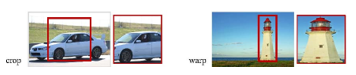Figure 1: Cropping and warping. This image is from [6]

In [22], super-resolution is said to construct high-resolution images by adding of new pixels which have high frequency components to the neighbor pixels, instead of adding simply computated new pixels. The frequency components are from multiple observed low-resolution images or from a single low-resolution image.

There are four categories in super-resolution algorithms such as prediction, edge-based, statistical, and example-based methods. Among them, the space-coding based method, which is a kind of example-based method, is popular nowadays.

Let  denote the high-resolution image desired and  be the kth low-resolution observation. Assume the image system captures iteratively k low-resolution images of , where the low-resolution iterations are related with the high-resolution image  by

where  represents the geometric warp (motion information) on the X,  is the linear space-variant blurring effects,  is the down-sampling decimation operator, and  is the additive zero-mean Gaussian noise. Equation (1) can be represented in matrices or equivalently, .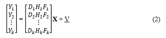

The obtained model (2) is a classic restoration, and the Expectation-Maximization (EM) estimator or the MAP can be applied in order to restore the image X. Similarly to the above image observation model, statistical approaches in [23] relate the super-resolution restoration steps in iteration toward optimal restoration. Therefore, the super-resolution reconstruction is cast into a full Bayesian framework, and by sum rule and Bayes’ theorem. Finally, if we can estimate W, then X can be obtained as a popular maximum a posteriori (MAP), or X can even be reduced to the simplest maximum likelihood (ML) estimator, which can be treated by an Expectation-Maximization (EM) algorithm in machine learning.

In [24], two kinds of super-resolution algorithms are introduced. Compared with the multiple-image super-resolution algorithm, the single image super-resolution algorithm uses a training step for the relationship between a set of high-resolution images and their low-resolution equivalents. This relationship is then used to predict the missing high-resolution components of the input images. There are three steps in this process: the registration (motion estimation), the restoration, and the interpolation to construct a high-resolution image from a low-resolution image or multiple low-resolution images [25].

In addition to the EM algorithm for single image super-resolution, [26]-[25] present methods that employ a mixture of experts (MoE) to jointly learn the features by separating global and local models (space partitioning and local regressing). These are solved by an expectation and maximization (EM) for joint learning of space partitioning and local regressing. Generative Adversarial Networks (GAN) method in [29] is proposed using generative networks and discriminative networks to restore most likely original images with reducing of the mean squared reconstruction error.

In this paper, we will apply a single image super-resolution method to get better detection rates from a single image dataset.

3. Image Resolution Improvements

There are two approaches to improving input image quality. The first is to apply the super-resolution directly to the input images then have the CNN take the super-resolution image as the input image. The second is to apply the super-resolution only to bounding boxes. The second method may reduce the necessary computing power.

Shaoqing Ren et al. [4] implemented the interpolation algorithm for two purposes. One was to fix the input image size from variable input images, and the other was for the selective search algorithm to extract feature maps from input images.  Detector extends networks for windowed detection by a list of crops or selective search (or EdgeBoxes) feature maps and then interpolates them to fix the size into one of the bounding boxes. Thus, this method may have more effects on bounding boxes for small objects, as shown in Figure 2. In [6], this method was described in detail in Section 4. In future research, we will implement CNN with extended images which are preprocessed using the super-resolution method instead of interpolation. In this paper, we propose using super-resolution as pre-processing before CNN to increase the image size to approximately 492×324 pixels.

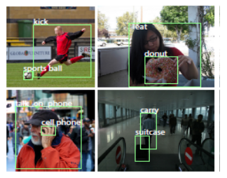Figure 2: Images with either full-size objects or small-sized objects. These examples are from [30]

Thus, we will first describe a single image super-resolution method to enhance the quality of the image in preprocessing before forwarding image data to the input layer of CNN. Then, it is followed by the CNN algorithm to classify preprocessed images.

3.1.  Super-resolution as Pre-processing

In image analysis, there have been distinct improvements related to convolution neural networks. However, we will focus on preprocessing image samples by super-resolution methods. For example, if a cropped 166×110 pixel image is extracted from a larger image of 640×480 pixels, the cropped image is usually too small to feed into the input layer of CNN models to get good results in object recognition. Thus, we will import a super-resolution method before the input layer of CNN or for bounding boxes.

We propose a Mixture of Experts (MoE) model to solve problems in anchor-based local learning, which are optimizing the partition of feature space and reducing the number of anchor points. The MoE model will be solved by Expectation-Maximization (EM) algorithm. The objective of a MoE model is to partition a large complex set of data into smaller subsets via the gating function. This preprocessing is built with the lazy neighbor embedding, anchor-based local learning approach, sparse coding, and deep convolution neural networks, respectively.

Component regressors, , and an anchor point,  have the following relationship as an expert which means that each of the model component classifiers or regressors is highly trained:where  is a low resolution path,  is the corresponding high resolution patch,  is the nearest anchor point for  and  is a continuous scalar value which represents the degree of membership of .

However, we propose a mixture of experts, which is one of the conditional combined mixture models in [31][32], in order to partition an image data into smaller subsets (as gating networks to determine which components are dominant in the region) and to determine the best (as experts to make predictions in their own regions).

In general, this a mixture of experts model can be trained efficiently by maximum likelihood using the EM algorithm in the M step. For every iteration, the posterior probabilities are calculated and reweighted for patches, and then we get LR/HR patch pairs  through the expectation of the log-likelihood as an E-step. During M-step, anchor points and regressors are updated, which is a softmax regression problem. After training, which is saving the trained anchor points and the projection matrices, a super-resolution image from the given input low-resolution image can be constructed by collecting all the patches from regressed low-resolution patches and averaging the overlapped pixels.

In order to compare the performance of our proposed method with that of interpolation methods, in addition to images produced by the super-resolution method, bilinear and bicubic interpolated images will also be generated.

3.2.  Object classification

As the object classification model, we decided to implement the CNN mostly based on the Faster R-CNN [4] because these networks support variable image sizes as the input data of CNN and sliding widow proposal scanning for the convolution network. Most importantly, the detection speed to predict an object is almost as fast as real-time. In YOLO or SSD, a group of an object can be detected, and the Faster R-CNN is enough to meet our goal. As mentioned earlier, Faster R-CNN uses the region proposal approach to detect an object from variable input image sizes. But the size ratio of the region proposal to the whole image is critical to detect the object. As shown in Figure 2, sometimes objects from small bounding boxes are ignored because the object may be deformed or aliased during cropping or warping. With a better quality image, CNN will make better quality cropped or warped bounding boxes. This means we can distinguish our proposed method from other interpolated data.

As the pre-processing, the super-resolution is implemented on MATLAB on Linux and Intel® Xeon. Our proposed neural networks are implemented in two ways. For one example, CNN is implemented only on Intel® Xeon CPU 2.30GHz, and as another example, CNN is implemented based on Intel® Xeon CPU 2.30GHz and eight GPUs in four NVIDIA Tesla K80 GPU boards. Since our purpose is not to find how fast objects are detected but rather how many objects are detected, we do not discuss these different platforms anymore.

Our proposed CNN has built to predict region proposals in terms of region proposal networks (RPN), which are implemented by deep convolution networks (a kind of fully convolutional network  [6]) [2][8]. This RPNs can predict region proposals with wide ranges of input image sizes and aspect ratios in contrast to conventional neural networks. The RPN also runs on pyramids of regression references (or pyramid of anchors), not on pyramids of images. It has benefits on running speeds.

The detection modules are organized as below: Multiple convolution layers convolve an input image and output feature maps. Then feature maps are given to the RPN. The RPN, in terms of a sliding window with a Multi-boxing method, generates a set of rectangular object proposals as a deep, fully convolutional network. A wide range of input image scales is fixed into given anchor sizes. After the RPN, conventional CNN predicts objects using the classification layer and bounds a box around the detected object using the regression layer.

In addition, for the storage usage of CAFFE, we make constraints on reading input images from the given image dataset. In our deep CNN model allowing multiple scaled image sizes, the maximum number of region proposals is w (the width of the image) multiplied by h (the height of the image) multiplied by k (the number of anchors of a region proposal). This means that the region proposal network requires a considerable amount of memory space. Therefore, we limited the feeding of the number of input images in hidden layers to less than or equal to 20 simultaneous images. Other than CAFFE, we used a version of the Keras model, which uses Tensorflow and GPUs. This other implementation had similar results. Therefore, we will not discuss it in this paper.

For the training of our CNN model, we use model parameters given in [4], which are actually initialized by pre-training model parameters of ImageNet. We test 9000 images from datasets with PASCAL VOC 2007 and also tests with Microsoft’s COCO dataset. As we said before, we consider more only on the number of detected objects but not the improving or computational speeds. Therefore, we are pretty sure that our model training procedure is adequately fitted to our purpose.

For each region proposal from an input image, an object is randomly counted on, and we randomly sample 256 anchors in an image as a mini-batch size. Instead of considering the super-resolution method on selected region proposals instead of interpolation methods, any input images with variable sizes or shapes can be supported with better cropped or warped regions. But we do not consider this right now. We will leave this for future research. Instead, we processed with low-resolution images as the input dataset, processing super-resolution on these images, then detecting objects.

4. Performance Evaluations

To detect objects from images in CNNs, there are two kinds of popular file formats as input datasets. Those formats are JPG and Bitmap. However, we have considered several more image file formats as well as JPG and Bitmap formats to get better image quality for preprocessing and to get better detection objects during testing images. While datasets such as PASCAL VOC2007 or COCO are generated images with the JPG file format, in super-resolution processing, the JPG format did not seem to offer results as good as the Bitmap format. Such effects on preprocessing, we decided to use Bitmap format, and then we worked to convert the images from JPG format into BMP format before a preprocessing procedure. Also, we scaled down the image size, reducing each width and height by a factor of three to generate images of lower quality, instead of directly collecting cropped or warped images. Then, the image was further processed with bilinear and bicubic interpolations, as well as the super-resolution method. Thus, we built three different image datasets as preprocessing in our proposed method.

In our model, we implemented the preprocessing procedure based on [26]. Rather than training with nearly 50 images as in most of the published single image super-resolution models, we trained our model based on their initial parameters and with 100 PASCAL VOC2007 images and COCO images. We did not find any considerable overfitting with this number of training images. We generated images as the preprocessing of our method with randomly selected images from PASCAL VOC2007 [16][33], images from [34], and additionally with the COCO dataset images. Newly built images after our preprocessing are similar categories and the number of objects in an image. Therefore, we tested the object classification with 520 images randomly extracted from VOC2007 and 1224 images from COCOs MSO [35].

As shown in Figure 3, we knew that the dataset was annotated with a different number of objects compared to our intuition, and our proposed model found it. For example, the first image of Figure 3 was annotated with no number of any designated object, but our proposed model caught an object or several objects, as shown in the image. The second image of Figure 3 shows that a sofa was detected even though the image was annotated with no object. Because of these differences, we decided to use roughly the given annotations from the given dataset. A larger number of people than the labeled number was detected in the third image of Figure 3. This meant that we needed to manually count the number of objects in each image in the dataset to get the precision-recall measures.

4.1.  Comparison of Output Pictures

Even though some of the images from the PASCAL VOC 2007 were  detected as   the   image   had no   objects in the   designated

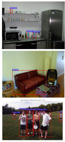Figure 3: Some Images labeled with no objects on annotated dataset but detected objects by our method.

categories, multiple objects in the categories are detected from almost all of the images, as shown in the results given in Table 10. There were three different preprocessing models, namely bilinear interpolation, bicubic interpolation, and our super-resolution method. After the preprocessing of input images, our model for object detection was set with a learning rate of 0.001 to train and detection scores with 0.8 or higher compared with ground truths (IoU) at the testing stage. Our model has 21 categories that are randomly selected and which are independent of each other.

As shown in Figure 4, Figure 5, and Figure 6, green color bars (the first column) show the number of detected objects in each category as given by bilinear interpolation, blue color bars (the second column) show the number as given by bicubic interpolation, and red color bars (the third column) show the results for our proposed approach. Both the number of objects detected as y-coordinate and the detection rate as x-coordinate are shown.

As shown in Table 1, our model detects more objects than the other two models, but the average detection scores are not very different. This demonstrates that our model generates improved input images of which objects had lower scores than 0.8 compared with ground truth images in the other two models, which are then fed into the CNN which is able to increase the number of detections of categories. Here we mean the detection score is the probability that the detected object belongs to the class. Therefore, objects with near- or over-threshold scores (80% or above) are included even though they did not get the scores over the threshold value in the bilinear or bicubic interpolation models. Figure 4 shows the number of detected objects from the PASCAL VOC 2007 dataset and the comparison between them.

In Table 1, Table 2, In Figure 7, our proposed model detects a chair which is quite a small object compared with the image size, while the other two models did not detect this ‘chair’ object. It is looked like that a small change by preprocessing before CNN can make a big difference. Even though the other chair, which is bigger than the chair, is detected in all three models, our proposed model has a little higher score. Thus, we can conclude our model can help to improve image qualities in image analyses. In particular, with video surveillance camera systems, our model may help to detect more objects. Therefore, we are interested in surveillance camera systems as a future research topic.

#tp means the number of correctly predicted objects (true positive), and the mean column shows the classification average probabilities predicted.

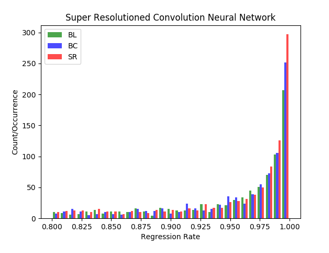Figure 4: Histogram for object detection models: images from VOC 2007 dataset.

With the dataset of Microsoft MSO as another image dataset for testing object classification, we present results in Figure 5 and Table 2. As with the VOC2007 dataset, our proposed model detects more objects than the two other models. This indicates that the image quality of low scored objects improved, leading to better detection. In other words, in our model, the image quality of low-scored objects improved, leading to detection scores (which is the probability that the object is the class) above 80%.

The main change in the COCO 2017 test dataset [36] is that instead of an 83K/41K train/validation split, the split is now 118K/5K for train/validation. Also, for testing, in 2017, the test set only had two splits (dev / challenge), instead of the four splits (dev / standard / reserve / challenge) used in previous years. For training of this dataset, we followed similar procedures as we did in PASCAL VOC 2007. For this dataset, we present the results in Figure 6 and In Figure 7, our proposed model detects a chair which is quite a small object compared with the image size, while the other two models did not detect this ‘chair’ object. It is looked like that a small change by preprocessing before CNN can make a big difference. Even though the other chair, which is bigger than the chair, is detected in all three models, our proposed model has a little higher score. Thus, we can conclude our model can help to improve image qualities in image analyses. In particular, with video surveillance camera systems, our model may help to detect more objects. Therefore, we are interested in surveillance camera systems as a future research topic.

. The total number of detected objects using our model was much bigger than the bilinear or bicubic models. However, the mean probabilities of detected objects were similar or a little bit lower. This indicates that many objects which were not detected with bilinear or bicubic interpolation methods were detected with our method.

Table 1: The number of detected objects on each category and the prediction scores on three different preprocessing and CNN with the PASCAL VOC2007 dataset.

	Bilinear		Bicubic		Our Method
Classes	#tp	mean	#tp	mean	#tp	mean
aeroplane	25	0.9569	29	0.9472	27	0.9787
bicycle	16	0.9602	17	0.9697	18	0.9520
bird	18	0.9204	25	0.9178	30	0.9500
boat	16	0.9330	18	0.9260	20	0.9276
bottle	19	0.9222	17	0.9208	15	0.9331
bus	26	0.9626	25	0.9639	26	0.9588
car	93	0.9662	100	0.9671	104	0.9710
cat	11	0.9427	10	0.9665	11	0.9739
chair	25	0.9273	34	0.9368	45	0.9320
cow	11	0.9149	12	0.9216	16	0.9385
dining table	7	0.9317	7	0.9420	12	0.9193
dog	37	0.9559	36	0.9657	35	0.9565
horse	30	0.9560	34	0.9574	37	0.9694
motorbike	13	0.9467	13	0.9630	16	0.9581
person	405	0.9546	432	0.9575	466	0.9590
potted plant	10	0.9467	12	0.9194	18	0.8767
sheep	15	0.9275	13	0.9380	14	0.9227
sofa	7	0.9191	8	0.9175	8	0.9475
train	7	0.9193	4	0.9276	4	0.9572
tvmonitor	25	0.9653	25	0.9729	26	0.9479
Total	816	0.9415	871	0.9450	948	0.9465
misclassified	25		21		39

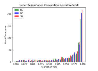Figure 5: Histogram for object detection models: images from the MSO dataset.

4.2.  Big vs. Small ROI Pictures and Their Detection Rates

As mentioned above, if an object is sufficiently large relative to the size of the image which contains the object in a region proposal, objects from interpolated images with bilinear or bicubic methods are identified satisfactorily and sometimes may have better perfor mance means that there is a higher probability that the object is identified as being in the specified class. However, the model we have proposed obtains much better results when the objects are from small bounding boxes, or if there is a small ratio of object size to the size of the image which contains the object (it means small anchor boxes in region proposals).

Table 2: The number of detected objects on each category and the prediction scores on three different preprocessing and CNN with the MSO dataset.

	Bilinear		Bicubic		Our Method
Classes	#tp	mean	#tp	mean	#tp	mean
aeroplane	5	0.9650	6	0.9300	9	0.9263
bicycle	1	0.9992	2	0.9112	1	0.9978
bird	50	0.9512	59	0.9521	75	0.9627
boat	1	0.8301	1	0.9771	1	0.9713
bottle	23	0.9074	24	0.9062	21	0.9117
bus	3	0.9954	3	0.9954	3	0.9871
car	16	0.9641	19	0.9558	18	0.9499
cat	11	0.9639	10	0.9829	11	0.9540
chair	19	0.9299	20	0.9270	22	0.9393
cow	5	0.9452	6	0.9488	7	0.9584
dining table	3	0.9410	4	0.8927	4	0.9072
dog	42	0.9559	47	0.9636	50	0.9478
horse	11	0.9728	11	0.9726	15	0.9362
motorbike	4	0.9487	4	0.9529	4	0.9588
person	302	0.9715	318	0.9718	340	0.9719
potted plant	4	0.9023	5	0.8756	9	0.9035
sheep	1	0.8780	1	0.9353	4	0.9064
sofa	3	0.9204	3	0.9099	6	0.9261
train	6	0.9746	7	0.9529	8	0.9522
tvmonitor	6	0.9720	6	0.9804	10	0.9248
Total	516	0.9444	556	0.9447	618	0.9447
misclassified	86		82		92

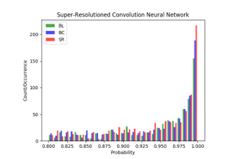Figure 6: Histogram for object detection models: images from COCO 2017 dataset.

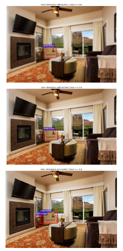Figure 7: Examples of small object scales through three models

In Figure 7, our proposed model detects a chair which is quite a small object compared with the image size, while the other two models did not detect this ‘chair’ object. It is looked like that a small change by preprocessing before CNN can make a big difference. Even though the other chair, which is bigger than the chair, is detected in all three models, our proposed model has a little higher score. Thus, we can conclude our model can help to improve image qualities in image analyses. In particular, with video surveillance camera systems, our model may help to detect more objects. Therefore, we are interested in surveillance camera systems as a future research topic.

5. Conclusion

Our proposed model appears particularly powerful in three scenarios; firstly, where there are relatively small objects in large pictures; secondly, where there is warping in the region proposals approach; and finally, with object detection from cropped images. Commonly, there are many noisy video images from surveillance camera systems, especially with night vision systems. Our method will remove a significant amount of aliased or mosaicked areas in these images, and so help to detect more objects. We compared our scheme with other approaches on three datasets showing an increased object in each case.

In future work, we will implement the super-resolution method confined to the bounding box areas. This will reduce the needed computational resources and allow us to use this method in real-time processing [37] and achieve better object recognition in this application. We will demonstrate this capability using modern streaming software environments [38].

Table 3: The number of detected objects on each category and the prediction scores on three different preprocessing and CNN with the COCO 2017 dataset.

	Bilinear		Bicubic		Our Method
Classes	#tp	mean	#tp	mean	#tp	mean
aeroplane	9	0.9652	10	0.9502	11	0.9684
bicycle	1	0.8821	2	0.9012	3	0.9250
bird	5	0.9471	10	0.9066	17	0.9277
boat	5	0.9002	5	0.8908	7	0.8896
bottle	20	0.9116	25	0.9100	19	0.9160
bus	15	0.9725	16	0.9590	15	0.9456
car	24	0.9503	29	0.9251	28	0.9388
cat	6	0.9274	7	0.9235	10	0.9075
chair	26	0.9193	28	0.9169	36	0.9174
cow	12	0.9190	14	0.9287	14	0.9384
dining table	10	0.8989	9	0.9049	9	0.9063
dog	12	0.9184	12	0.9183	12	0.9047
horse	7	0.9219	8	0.9293	6	0.9402
motorbike	11	0.9604	14	0.9550	18	0.9368
person	411	0.9547	460	0.9521	498	0.9534
potted plant	16	0.8806	11	0.8824	15	0.9002
sheep	2	0.9585	2	0.9880	2	0.9977
sofa	3	0.9398	3	0.9015	2	0.8760
train	9	0.9358	10	0.9269	9	0.9427
tvmonitor	26	0.9461	24	0.9457	25	0.9544
Total	734	0.9305	805	0.9258	869	0.9293
misclassified	104		106		113

Acknowledgment

This work was supported by the 2017 sabbatical year research grant of the Korea Polytechnic University.

Geoffrey Fox was partially supported by NSF CIF21 DIBBS 1443054 and NSF CINES 1835598. We thank the Futuresystems group for the computational resources.

1. Bokyoon Na, Geoffrey Fox, “Object Detection by a Super-Resolution Method and a Convolutional Neural Networks”, IEEE International Conference on Big Data (Big Data) (2018)
2. Alex Krizhevsky, Ilya Sutskever, Geoffrey E. Hinton. “ImageNet Classification with Deep Convolution Neural Networks”. In Advances in Neural Information Processing Systems (NIPS), (1097-1105). (2012).
3. Girshick Ross. “Fast R-CNN”. arXiv: 1504.08083v2 [cs.CV] 27 Sep 2015.
4. Shaoqing Ren, Kaiming He, Ross Girshick, and Jian Sun. “Faster R-CNN: Towards Real-time Object Detection with Region Proposal Networks”. arXiv:1506.01497v3[cs.CV] 6 Jan 2016.
5. David Berthelot Schumm, Luke Metz Thomas. “BEGAN: Boundary Equilibrium Generative Adversarial Networks”. arXiv: 1703.10717v2 [cs.LG]. (2017).
6. Keiming He, Xiangyu Zhang, Shaoqing Ren, and Jian Sun. “Spatial Pyramid Pooling in Deep Convolutional Networks for Visual Recogniton”. arXiv:1406.4729v4. (2015).
7. Ross Girshick, Jeff Donahua, Trevor Darrell, Jitendra Malik, “Region-Based Convolution Networks for Accurate Object Detection and Segmentation”, IEEE Transactions on Pattern Analysis and Machine Intelligence Vol. 38, NO.1, 2016.
8. Karen Simonyan, Zisserman Andrew. “Very Deep Convolutional Networks for Large-Scale Image Recognition”. ICLR. (2015).
9. Joseph Redmon, Santosh Divvala, Ross Girshick, Ali Farhadi, “You Only Look Once: Unified, Real-time Object Detection”, The IEEE Conference on Computer Vision and Pattern Recognition (CVPR), 2016, pp. 779-788
10. Kaiming He, Georgia Gkioxari, Piotr Dollar, Ross Girshick, “Mask R-CNN”, The IEEE International Conference on Computer Vision (ICCV), 2017, pp. 2961-2969
11. Ghosh Nachum and Debiprasad Ofir. https://www.quora.com. “What-are-Generative-Adversarial-Networks-GANs”.
12. Tim Salimans Goodfellow, Wojciech Zaremba, Vicki Cheung Ian. “Improved Techniques for Training GANs”. arXiv:1606.03498v1. (2016).
13. Takeru Miyato M Dai, Ian Goodfellow Andrew. “Adversarial Training Methods for Semi-Supervised Text Classification”. ICLR. (2017).
14. Ian J. Goodfellow Pouget-Abadie, Mehdi Mirza, Bing Xu, David Warde-Farley, Sherjil Ozair, Aaron Courvill, Yoshua BengioJean. “Generative Adversarial Nets”. arXiv:1406.2661v1. (2014).
15. Sara Sabour, Nicholas Frosst, Geoffrey E. Hinton, “Dynamic Routing Between Capsules”, Advances in Neural Information Processing Systems 30 (NIPS 2017)
16. Everingham Van Gool, C. K. I. Williams, J. Winn, and A. ZissermanL. “The PASCAL Visual Object Classes Challenge 2007 (VOC2007) Results”. (2007).
17. Achanta R., Estrada F., Wils P., Süsstrunk S. “Salient Region Detection and Segmentation”. In: Gasteratos A., Vincze M., Tsotsos J.K. (eds) Computer Vision Systems. ICVS 2008. Lecture Notes in Computer Science, vol 5008. Springer, Berlin, Heidelberg. (2008)
18. Volodymyr Mnih, Nicolas Heess, Alex Graves, and Koray Kavukcuoglu. “Recurrent Models of Visual Attention”. arXiv:1406.6247v1[cs.LG] 24 Jun 2014.
19. Jimmy Lei Ba, Volodymyr Mnih, and Koray Kavukcuoglu. “Multiple Object Recognition with Visual Attention”. arXiv:1412.7755v2[cs.LG] 23 Apr 2015.
20. Karol Gregor Danihelka, Alex Graves, Danilo Jimenez Rezende, Daan Wierstra Ivo. “DRAW: A Recurrent Neural Network For Image Generation”. arXiv:1502.04623v2[cs.CV] 20 May 2015.
21. R.R. Uijlingsvan de Sande, T. Gevers, and A.W.M. Smeulders K.E.A. “Selective Search for Object Recognition”. IJCV. (2012).
22. Michael Elad, Arie Feuer, “Restoration of a Single Superresolution Image from Several Blurred, Noisy, and Undersampled Measured Images”, IEEE Transactions on Image Processing, Vol. 6, No. 12, December 1997
23. Jianchao Yang, John Wright, Thomas S. Huang, and Yi Ma, “Image Super-Resolution Via Sparse Representation”, IEEE TRANSACTIONS ON IMAGE PROCESSING, VOL. 19, NO. 11, pp2861, NOVEMBER 2010
24. Nasrollahi Kamal, Guerrero Escalera Sergio, Rasti Pejman, Anbarjafari Gholamerza, Baro Xavier, J. Escalante Hugo, Moeslund B. Thomas. “Deep Learning based Super-Resolution for Improved Action Recognition”. In International Conference on Image Processing Theory, Tools and Applications (IPTA) IEEE Signal Processing Society. (2015).
25. Brian C. Tom, Aggelos K. Katsaggelos, Nikolas P. Galatsanos. “Reconstruction of a high resolution image from registration and restoration of low resolution images”. In Proceedings of IEEE International Conference on Image Processing, pages 553-557, 1994
26. Kai Zhang Wang, Wangmeng Zuo, Hongzhi Zhang, Lei ZhangBaoquan. “Joint Learning of Multiple Regressors for Single Image Super Resolution”. IEEE Singnal Processing Letters. Vol. 23 No. 1. (2016).
27. Zhaowen Wang Liu, Jianchao Yang, Wei Han, Thomas Huang Ding. “Deep Networks for Image Super Resolution with Sparse Prior”. ICCV. (2015).
28. Chao Dong Change Loy, Kaiming He, Xiaoou Tang Chen. “Image Super Resolution Using Deep Convolution Networks”. arXiv:1501.00092v3.v (2015).
29. Christian Ledig Theis, Ferenc Huszar, Jose Caballero, Andrew Cunningham, Alejandro Acosta, Andrew Aitken, Alykhan Tejani, Johannes Totz, Zehan Wang, Wenzhe ShiLucas. “Photo-Realistic Single Image Super Resolution Using a Generative Adversarial Network”. arXiv:1609.04802v5[cs.CV]. (2017).
30. Georgia Gkioxari, Ross Girshick, Piotr Dollár, Kaiming He, “Detecting and Recognizing Human-Object Interactions”, The IEEE Conference on Computer Vision and Pattern Recognition (CVPR), 2018, pp. 8359-8367
31. Bishop Christopher. “Pattern Recognition and Machine Learning”. Springer. (2006).
32. Zhang Zhang, Baoquan Wang, Wangmeng Zuo, Hongzhi ZhangKai. “Joint Learning of Multiple Regressors for Single Image Super-Resolution”. IEEE Signal processing letters, Vol. 23, No.1. (2016).
33. Olga Russakovsky Deng, Hao Su, Jonathan Krause, Sanjeev Satheesh, Sean Ma, Zhiheng Huang, Andrej Karpathy, Aditya Khosla, Michael Bernstein, Alexander C. Berg and Li Fei-Fei Jia. “ImageNet Large Scale Visual Recognition Challenge”. arXiv:1409.0575. (2014).
34. Olga Russakovsky Deng, Hao Su, Jonathan Krause, Sanjeev Satheesh, Sean Ma, Zhiheng Huang, Andrej Karpathy, Aditya Khosla, Michael Bernstein, Alexander C. Berg and Li Fei-Fei Jia, “ImageNet Large Scale Visual Recognition Challenge 2017″. (2017).
35. Zhang Ma, Shuga Sameki, Mehrnoosh Sclaroff, Stan Betke, Margrit Lin, Zhe Shen, Xiaohui Price, Brian Much, Radom Jianming. “Salient Object Subitizing”. IEEE Conference on Computer Vision and Pattern Recognition (CVPR). (2015).
36. Tsung-Yi Lin, Michael Maire, Serge Belongie, Lubomir Bourdev, Ross Girshick, James Hays, Pietro Perona, Deva Ramanan, C. Lawrence Zitnick, Piotr Dollár. “Microsoft COCO: Common Objects in Context”, arXiv:1405.0312 [cs.CV]
37. Xinyuan Huang, Geoffrey C. Fox, Sergey Serebryakov, Ankur Mohan, Pawel Morkisz, Debojyoti Dutta, “Benchmarking Deep Learning for Time Series: Challenges and Directions“, Stream-ML workshopat IEEE Big Data Conference, Los Angeles CA December 10, 2019
38. Vibhatha Abeykoon, Supun Kamburugamuve, Kannan Govindrarajan,  Pulasthi Wickramasinghe, Chathura Widanage, Niranda Perera, Ahmet Uyar, Gurhan Gunduz, Selahattin Akkas, Gregor Von Laszewski, and Geoffrey Fox, “Streaming Machine Learning Algorithms with Big Data Systems”, Stream-ML workshopat IEEE Big Data Conference, Los Angeles CA December 10, 2019

(Click Here)

(Click Here)