1. Introduction

The Poisson k ∈ N (discrete) and standard Gamma x ∈ R⁺ (continuous) random variables are characterized by the asymmetric probability distributions:

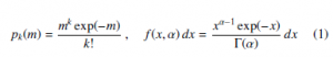
which depend on a single dimensionless parameter m ∈ R⁺ or α ∈ R⁺. The parameter coincides with both average and variance of the random variables while the skewness asymmetry parameter, equal to m^{− 1}₂ for the Poisson and 2α^{− 1}₂ for the Gamma distributions, tends to zero in the limit of large parameter values. Correspondingly both random variables weakly approach to a Gaussian limit for m → ∞ or α → ∞. These distributions are useful for the description of several phenomena involving Poisson and other random processes relevant to fundamental and applied research fields. The distributions share the same functional form with the roles of variable and parameter exchanged and therefore are also a representative example of conjugate a priori in the Bayesian formalism [1].

The availability and evolution of computing hardware [2]-[3] and the development of computational methods requiring the repeated generation of random numbers according to these distributions has stimulated the development of accurate and fast algorithms.

Most of these algorithms are based on different implementations of the rejection method, random variable transformations or their combination [4]. Exact algorithms for the generation of random numbers for the Poisson, Gamma, Beta and Binomial distributions were early introduced by Ahrens and Dieter [5], while specific improved algorithms for the Gamma [6, 7] and Poisson [8]-[13] random numbers have been extensively discussed. Versatile fast algorithms for repeated extractions of random numbers from the same discrete distribution (also Poisson with parameter m) were developed by Marsaglia and co-workers [14]. They are based on the random access to suitable pre-calculated tables that contain the integers to be generated in such a way that they are drawn with the desired probability.

Approximate methods often provide useful alternatives especially when a wide range of large parameter values are encountered. The large-parameter Gaussian limit for the Poisson and Gamma distributions suggests the possibility to generate approximate random numbers with linear transformations of the type:

from a standard Gaussian random number z generated using well established approaches. It can be expected that more complex non-linear transformations may provide more efficient strategies to exploit the Gaussian random number z. In the historical paper by Wilson and Hilferty (WH) [15] non-linear transformations of the form x = (a + bz)^p were investigated to provide approximate confidence intervals for the χ² random variable (a Gamma with semi-integer parameters) from the Gaussian confidence intervals. A useful transformation was obtained using p = 3.

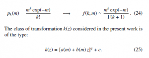
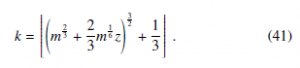
The possibility to use the WH transformation to approximate the Poisson cumulative distribution was recently emphasized in a paper of Lesch and Jeske [16] exploiting a relationship between the Gamma and Poisson random variables through the cumulative distribution function. In this paper, considering P_k(m) as the Poissonian cumulative distribution function, and Φ(x) the Gaussian cumulative distribution function, the following approximation is stated:

k . Since the Eq. (3) is not explicable with a formula which expresses the Poisson as dependent variable of a Gaussian variable, an explicit non-linear transformation is still missing according to our knowledge.

In this paper we are interested in finding a non-linear transformation for the Poisson random variable exploiting the Gaussian random variable, in the spirit of the WH approach used for the Gamma random variable [15, 7]. Our interest in the generation of Poisson random numbers was motivated by the effort to develop a Kinetic Monte Carlo computer simulation of the classical nucleation process [17] and was required for an approximate treatment of the high transition rate region. The method has been recently applied to compute the homogeneous crystalline nucleation rate in undercooled liquid Ni [18] for comparison with experimental data. In the parameter range m ≤ 50, an efficient exact approach was adopted combining the method of Marsaglia [14], tabulated for integer parameter values, with a O(m) algorithm correction for the decimal part of m. While, for larger m, the following non-linear transformation from a standard Gaussian random number z, was adopted:

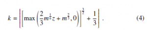
Eq. (4), that has apparently never been suggested before, was introduced in a previous paper without derivation [17]. In this paper an analytic justification for the above expression is illustrated. It will be shown that this approximation can be obtained with an approach analogous to WH transformation for the Gamma random variable. The aim is to find the optimal transformation in a given class of functions for which the Taylor expansion about the maximum of the logarithm of the transformed probability density, is closer to a parabolic shape. It is believed that this transformation can be useful in many applications requiring an efficient generation of Poisson random numbers with parameters m & 10 (variable in a wide range) and represents a good trade off between computing time and accuracy.

The paper is organized as follows. In Sec. 2 the WH transformation and a higher order formula for the Gamma distribution are presented. Furthermore, approximations to the Gamma function are discussed in the same section, exploiting the two transformation. The non-linear transformation method is extended to the Poisson distribution in Sec. 3 and the previous transformation (4) established. The approximation errors on the cumulative and probability distributions are investigated in Sec. 4. Conclusions are drawn in Sec. 5.

2. Considerations on WH-type Approximations for the Gamma Random Variable and Gamma Function

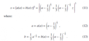
The original WH paper [15] is focused on the Gamma random variable whose probability density is f(x,α) in Eq. (1), related to the Erlang (α ∈ Z⁺), and χ² (2α ∈ Z⁺) distributions. The spirit of the original approach is to look for a non-linear transformation of the type:

where x is the Gamma random variable, z is the transformed random variable, and a, b and p are suitable constants to be determined in such a way that z is closely approximated by a standard Gaussian random variable. The original WH approach considers ψ(z) = 0, but it is possible to extend the class of transformations including an analytic correction ψ(z) with ψ(0) = 0, ψ⁰(0) = 0, ψ⁰⁰(0) = 0. Throughout this paper the Lagrange’s primes notation will be used and the successive derivatives of f(x) are indicated as f⁰(x), f⁰⁰(x), f000(x), f(4)(x), f(5)(x)

The differentials dx and dz of the original and transformed random variables, according to Eq. (1), are related by:

in order to recall a parabolic shape and therefore a Gaussian density function for g(z,α) in the neighborhood of the peak z = 0.

In the simplest case, corresponding to the original WH transformation [15], where ψ(z) = 0, it is demonstrated that Eq. (5) is:

Always in the WH demonstration [15], the parameter p results p = 3. This choise is endorsed by the fact that p = 3 implies that

φ⁰⁰⁰(0) = 0 for a wide class of ψ(z) functions where ψ⁽⁴⁾(z) = 0, which is obviously true for ψ(z) = 0.

It is possible, however, to find transformations which improve the parabolic approximation for φ(z) imposing the additional condition φ⁽⁴⁾(0) = 0 to the others showed in Eq. (10). A good choice is to adopt a cubic ψ(z) term of the type:

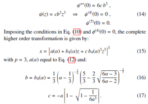
Furthermore, the previous Gaussian approximation to the transformed Gamma distribution (7) can be used to compute approximately the integral corresponding to the Γ(α) function in the spirit of the saddle point integration approach:

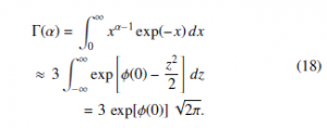
With respect to the usual Stirling approximation, the two non-linear transformations (11) and (15) produce integrand functions of z better approximated by a standard Gaussian. Recalling that:

the following approximations Γ_WH(α) and Γ₄(α) to the Γ(α) function are obtained:

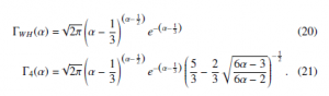
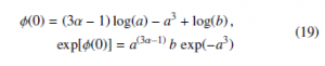
The modulus of the relative error (α) = 1 ^{− Γ}_Γ^a₍⁽_α^α₎⁾ of the two previous above approximations Γ_a(α), is reported in Fig. 1 an compared to the Stirling formula and the Stirling series (with two terms):            !α−1 α p   − 1

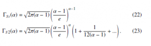
Figure 1: Relative error (α) of various approximations to the Γ(α) function. The curves refer to: the Stirling approximation Γ_St(α) (dot-dashed line), the WH approximation Γ_WH(α) (solid line), the higher-order WH approximation Γ₄(α) (dashed line), the first two terms of the Stirling series expansion Γ_S2 (dotted line). The thin straight line is a guideline for the eye corresponding to an α⁻² behaviour.

It is possible to notice that the approximations obtained by the WH approach (20) and (21) are better than the Stirling formula (22). In particular, the higher-order WH approximation (21) is characterized by a relative error decreasing as α⁻², similarly to the approximation obtained including the first two terms of the Stirling series (23).

3. The WH-type Approximation for the Poisson Distribution

The possibility to obtain an approximation to the Poisson cumulative distribution function, using a relationship between the Poisson and Gamma random variables (exploiting the application of the WH transformation to the latter) was emphasized [16]. In this approach the transformation z(k) for the Poisson distribution, cannot however be easily inverted to obtain an explicit k(z) relationship, analogous to the x(z) transformations for the Gamma distribution.

In this section an approach similar to the one mentioned in Sec. 2, and therefore referred to as a WH-type transformation, is applied to the Poisson distribution. Two additional complications arise: the first is that for a discrete random variable it is necessary to approximate the distribution with a continuous probability density, the second is the requirement to expand k! = Γ(k+1) at the denominator introducing an additional approximation. For these reasons there is no scope in pushing the expansion order while the accuracy of the final transformation will have to be numerically assessed. An advantage of the discrete nature of the approximated random variable is that the transformation will eventually inject finite z intervals into a single k value and the possible effects of the transformation singularity will be masked.

The simplest continuous approximation to the Poisson distribution (the approximate normalization is not relevant for the following arguments) is given by:

The opportunity to include an additional constant term c, with respect to (5) with ψ(z) = 0, is suggested by a flexibility requirement for the successive conversion into integer numbers. The general

form of (25) and the resulting optimal functional dependencies a(m), b(m) and exponent q, are expected to be compatible with relatively fast numerical computations.

The probability density of the transformed random variable is obtained as usual:

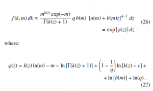
Similarly to the Gamma case treated in Sec. 2, the aim is to find the optimal parameters in such a way that the function ϕ(z) (27) at the exponent of the transformed probability density is close to a parabolic function in the neighbourhood of z = 0.

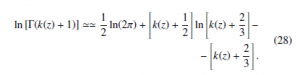
In order to calculate the derivatives of ϕ(z) respect to z, an explicit approximate functional expression for the logarithm of the Gamma function is required and, according to Eq. (20), it is possible to write:

An approximate expression for ϕ(z) (27) is obtained exploiting Eq. (28), retaining the leading terms in k ln(k), k, ln(k) and neglecting constants or lower order terms as: ϕ(z) ‘ −k(z)ln[k(z)] + k(z) + k(z)ln(m) −  ln[k(z)]+

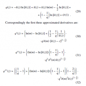
where further terms of order O(1) have been neglected in the second and third derivatives and the condition k(z)  c accounted for. The analytic conditions to be imposed to equations (30), (31) and (32) are that these first three derivatives of ϕ(z) in z = 0 should satisfy:

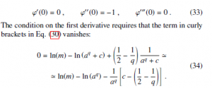
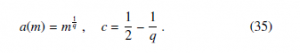
In this expression the identity k(0) = a^q + c was used and, considering that c  k ‘ a^q, the logarithm was expanded to the first order as ln(a^q + c) ‘ ln(a^q) + _a^c_q and the denominator in the last term approximated as a^q + c ‘ a^q. In order to satisfy Eq. (34) it is possible to chose:

By evaluating (31) in z = 0, considering that to the O(1) order ln(m)−ln[k(0)] ‘ 0 and the term in curly brackets is ‘ −1, imposing the condition ϕ⁰⁰(0) = −1, it is found that:

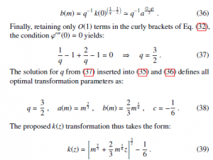
The performance and meaning of transformation (39) is illustrated in Fig. 2 for a typical Poisson distribution with a relatively low parameter value (m = 10). The small (∗) symbols are exact numerical results, reported at the ordinate integer values k and k + 1 and abscissa z such that the cumulative distributions of the Poisson random variable (up to k included) and of the standard Gaussian (up to z) coincide, that is:

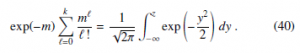
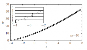
Figure 2: Relationship between the standard Gaussian z and Poisson k (parameter m = 10) random variables. Couples (z,k), (z,k + 1) (∗ symbols) where a matching between the corresponding cumulative distributions occurs, according to Eq. (40). Proposed non linear transformation (dashed curve) Eq. (39). Stepwise discretized transformation Eq. (41). The small k range is magnified in the inset.

The dashed curve is the approximate transformation (39) that clearly interpolates the numerical result for the exact discrete random variable. In order to use the continuous transformation to generate correctly integer values, a continuity correction has to be applied. This can be performed by adding a constant shift + to the transformation and taking the largest integral value that is not greater than the resulting real number^[1]. The discretized version of the transformation is therefore:

This expression corresponds to the stepwise curve reported in Fig. 2 that closely reproduces the exact numerical steps (symbols ∗) especially in the |z| < 3 high probability region. The remote possibility that a large negative z results in a negative k is overcome by the max operator in the final transformation, anticipated in Eq.

(4), that injects these cases in the k = 0 random number.

4 . Accuracy Assessment

Several statistical indicators can be considered to investigate the errors of the proposed approximation (4) in comparison with the linear transformation (2) or the one proposed in the paper of Chang [19] and of Lesch [16]. As described by Lesch [16], useful statistical indicators quantify the maximum deviations on both the probability and the cumulative distributions and can be defined respectively as the maximum absolute difference between the exact Poisson probability p_k and the approximate probability f_k,

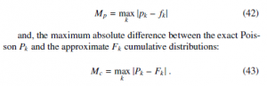
The dependence of these two indicators as a function of m is illustrated in Fig. 3 in double logarithmic plots, which quantifies the precision of the approximations.

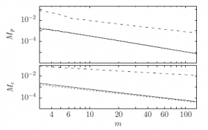
Figure 3: Double logarithmic plot of the dependence of the two statistical indicators

M_p (42) and M_c (43) as a function of the Poisson parameter m. The performance of the proposed non-linear transformation (solid lines) is compared with the linear transformation (dashed lines) and the transformation proposed by Lesch [16] (dotted lines). This latter curve overlaps with the solid line in the M_p case.

The behaviour of the two indicators are showed in each sub-plot for the linear (Eq. 2 with dashed line), the non-linear (Eq. 4 with solid line) and the Lesch transformations ([16] with dotted line). It is possible to notice that, for the non-linear transformation, the two indicators decrease with increasing m roughly as m^−1.5 in both the case. So, the performance of the proposed approximation (4) is substantially equivalent to the one proposed by Lesch [16] with the advantage of the availability of an explicit k(z) expression for the random number generation.

The χ² test is also performed and showed in Fig. 4 as a function of the sample number N. As in Fig. 3, the indicator is reported for three different number of degree of freedom nc (7, 57, 89), which correspond respectively to different values of the Poisson parameter m (1, 60.24, 144.89). The χ² value is reported for the linear (Eq. 2 with dashed line), the non-linear (Eq. 4 with solid line) and the Lesch transformations ([16] with dotted line). The horizontal line represents the χ² level of significance considered at 5%. Under the line, the hypothesis test is considered verified and the random numbers obtained through the transformation (4) are considered distributed as a Poisson function. This means that the approximation is good. Furthermore, its goodness improves with the increasing of the degree of freedom nc, and so with the increasing of the Poisson parameter m.

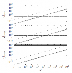
Figure 4: The dependence of the statistical indicator χ² as a function of the sample dimension N. The performance of the proposed non-linear transformation (solid lines) is compared with the linear transformation (dashed lines) and the transformation proposed by Lesch [16] (dotted lines). The plot are showed for three different case of degree of freedom nc, which correspond to different value of the Poisson parameter m. In particular for nc = 7 m = 1, nc = 57 m = 60.64 and nc = 89 m = 144.89. The horizontal line represents the level of significance of 5% taken from the χ² table under which the hypothesis of the χ² test is verified.

It is evident the better performance of the proposed non-linear transformation (solid line) respect to the linear one, furthermore, its goodness increases with the increasing of the degree of freedom.

As in the case of the previous statistical indicators, the proposed approximation (4) is substantially equivalent to the one proposed by Lesch [16].

5.  Conclusions

In this paper WH type non-linear transformation between a standard Gaussian random variable z and Poisson k random variable was investigated. The historical WH transformation, was revisited and its corresponding approximations to the Gamma function were investigated. The WH approach was extended to the Poisson random variable and a relatively simple transformation was established. The accuracy of the transformation was assessed as a function of the Poisson parameter m.

This result provide an analytic justification for the proposed transformation (4) to generate approximate Poisson random numbers for arbitrary parameter m introduced in the previous paper [17]. The proposed transformation has a relatively simple functional structure and can be implemented using fast library routines for the evaluation of square roots sqrt, while the slower pow function is not required. The execution of (4), including the generation of the Gaussian random number, requires about 53 ns on a 3.7 GHz 64-bit processor and the reliability of the generated random numbers is fully acceptable for m ≥ 10 for most applications. The improved reliability of the generated random number with respect_√ to the simpler linear transformation m + mz fully justifies the required additional 4 ns of computing time.

While a large number of exact methods for the generation of Poisson random number with different characteristics are described in the literature [8], [11]-[14], the present method is expected to provide a useful approximate alternative for several possible applications. Marsaglia’s method [14], for example, is useful for repeated extractions from the same distribution (parameter m), since different arrays are required if m changes. Our method for sure is slower and less precise (since it is an approximation) than the Marsaglia’s method, anyway it is a valid alternative for the cases where m varies over time, giving a good trade-off between precision computing speed. A possible application filed of the proposed algorithm is the filed of embedded systems and Wireless Sensor Networks (WSN)[20, 21], where the aspect just mentioned has its importance.

The method actually provides an explicit expression for the random number generation, implementing the ideas of the usage of the WH non-linear transformation recently emphasized in the educational literature [16]. Furthermore, this paper intend to be an hint for a more precise mathematical work in which to provide analytical bounds and how the proposed transformation is related to the central limit theorem. Finally, last observation, this method could be the basis for a new rejection method, increasing its random number generation accuracy.

Conflict of Interest

The authors declare no conflict of interest.

1. G. D’Agostini. Bayesian inference in processing experimental data: principles and basic applications. Reports on Progress in Physics, 66:1383–1419, 2003.
2. M. Faccio, F. Federici, G. Marini, V. Muttillo, L. Pomante, and G. Valente. Design and validation of multi-core embedded systems under time-to-prototype and high performance constraints. In 2016 IEEE 2nd International Forum on Research and Technologies for Society and Industry Leveraging a better tomor- row (RTSI), 2016. https://doi.org/10.1109/RTSI.2016.7740546.
3. V. Muttillo, G. Valente, F. Federici, L. Pomante, M. Faccio, C. Tieri, and
   S. Ferri. A design methodology for soft-core platforms on fpga with smp linux, openmp support, and distributed hardware profiling system. EURASIP Journal on Embedded Systems, 2016(1):15, Sep 2016. https://doi.org/10.1186/ s13639-016-0051-9.
4. L. Devroye. Non-Uniform Random Variate Generation. Springer, 1986.
   https://doi.org/10.1007/978-1-4613-8643-8.
5. J. H. Ahrens and U. Dieter. Computer methods for sampling from gamma, beta, poisson and bionomial distributions. Computing, 12:223–246, Sep. 1974. https://doi.org/10.1007/BF02293108.
6. G. Marsaglia. The squeeze method for generating gamma variates. Computers and Mathematics with Applications, 3:321–325, 1977. https://doi.org/ 10.1016/0898-1221(77)90089-X.
7. G Marsaglia and W. W. Tsang. A simple method for generating gamma vari- ables. ACM Transactions on Mathematical Software, 26(3):363–372, Sep. 2000. https://doi.org/10.1145/358407.358414.
8. G. S. Fishman. Sampling from the poisson distribution on a computer. Com- puting, 17:147–156, Jun. 1976. https://doi.org/10.1007/BF02276759.
9. A. C. Atkinson. The computer generation of poisson random variables. Journal of the Royal Statistical Society. Series C (Applied Statistics), 28:29–35, 1979. https://doi.org/10.2307/2346807.
10. A. C. Atkinson. Recent developments in the computer generation of poisson random variables. Journal of the Royal Statistical Society. Series C (Applied Statistics), 28:260–263, 1979. https://doi.org/10.1007/BF02243478.
11. L. Devroye. The computer generation of poisson random variables. Computing, 26:197–207, 1981. https://doi.org/10.1007/BF02243478.
12. C. D. Kemp and A. W. Kemp. Poisson random variate generation. Journal of the Royal Statistical Society. Series C (Applied Statistics), 40:143–158, 1991.
    https://doi.org/10.2307/2347913.
13. W. Hormann. The transformed rejection method for generating poisson ran- dom variables. Insurance: Mathematics and Economics, 12:39–45, Feb. 1993. https://doi.org/10.1016/0167-6687(93)90997-4.
14.  G. Marsaglia, W. W. Tsang, and J. Wang. Fast generation of discrete ran- dom variables. J. of Statistical Software, 11:1–11, July 2004. https:
    //doi.org/10.18637/jss.v011.i03.
15. E. B. Wilson and M. M. Hilferty. The distribution of chi-square. Proceed- ings of the National Academy of Sciences of the USA, 17:684–688, 1931. https://doi.org/10.1073/pnas.17.12.684.
16. S. M. Lesch and D. R. Jeske. Some suggestions for teaching about nor- mal approximations to poisson and binomial distribution functions. Journal of the American Statistical Association, 63:274–277, Aug. 2009. https:
    //doi.org/10.1198/tast.2009.08147.
17.  A. Filipponi and P. Giammatteo. Kinetic monte carlo simulation of the classical nucleation process. J. Chem. Phys., 145:211913, 2016. https:
    //doi.org/10.1063/1.4962757.
18. A. Filipponi, A. Di Cicco, S. De Panfilis, P. Giammatteo, and F. Iesari. Crys- talline nucleation in undercooled liquid nickel. Acta Materialia, 124:261–267, 2017. https://doi.org/10.1016/j.actamat.2016.10.076.
19. C. H. Chang, J. J. Lin, N. Pal, and M. C. Chiang. A note on improved approximation of the binomial distribution by the skew-normal distribu- tion. The American Statistician, 62(2):pp. 167–170, May 2008. https:
    //doi.org/10.1198/000313008X305359.
20. S. Marchesani, L. Pomante, M. Pugliese, and F. Santucci. Definition and development of a topology-based cryptographic scheme for wireless sen- sor networks. In Marco Zuniga and Gianluca Dini, editors, Sensor Systems and Software, pages 47–64, Cham, 2013. Springer International Publishing. https://doi.org/10.1007/978-3-319-04166-7_4.
21. L. Pomante, M. Pugliese, S. Marchesani, and F. Santucci. Winsome: A middle- ware platform for the provision of secure monitoring services over wireless sen- sor networks. 2013. https://doi.org/10.1109/IWCMC.2013.6583643.

(Click Here)

(Click Here)