1. Introduction and Literature Review

There could be many causes and variables for which a company does not obtain or maximize their profits. Some could be market competition, a lot, or little demand for products. However, for this research, we will focus on transportation costs that the company invests in distributing the products because the charge that generates to deliver the product to the final customer, is the expenses influence to the final price of the product, consequently in the business competitiveness.

For helping to reduce transportation costs, many companies choose to open more Distribution Centers (CEDIS). Ghiani et al. [1] define a Distribution Center as “the place mainly used in the large-scale distribution for the storage of products from different manufacturers, for distribution to the points of sale (and possibly another application belonging to the firm), located in a specific geographical area.” Moreover, their location must be analyzed to use as a strategy of cost reduction.

Because of opening, a CEDI is more expensive than opening a peripheral warehouse, and many companies take this option. Ghiani et al. [1] define a peripheral warehouse as “it is a warehouse served by a central warehouse and used for distribution of products to customers. Its objective is to ensure a better quality of customer service. Moreover, its operation cost is reduced because this warehouse only has an operational workforce.

There are many ways to select a correct place for the facility, but the competition and the technological innovation to this day make critical the use of different tools such as the use of Geographic Information Systems (GIS). Lo & Yeung [2] define GIS as “Computer-based systems specifically designed and implemented for two subtle but interrelated purposes, managing geospatial data, and using that data to solve spatial problems.” Church & Murray [3] also define a GIS as “A system of hardware, software, and procedures designed for decision making throughout the acquisition, administration, analysis, and output of spatially referenced information.”

For this study, we did an extensive search to know the applications of logistics, supply chain management, and GIS, finding a variety of applications implemented. One of the most common uses of GIS has been to support location sciences along with access to necessary spatial information, including the extraction of coordinates from location points and the attribute associated with a geographical location [4, 5].

Another case is in [6] where used GIS and Global Positioning System (GPS) to track assets within the supply chain, he cites the example of Walmart that avoid increasing the inventory costs or shortages of inventory using these technologies to curb these deficiencies giving them continuous monitoring your goods. Li et al. [7] demonstrated that genetic algorithms (GA) could be used with GIS to effectively solve spatial decision problems to locate optimal places to establish facilities using data such as population and transportation, apply GIS and solve it with GA where multiple objectives are incorporated to have as exit the best locations.

The application of GIS in recent years has been extended, whether in the public or private sector. It is due to this advance that logistics and supply chain management have found in this technology like such a promising future. [8] make use of the GIS procedures together with Multicriteria Analysis (MCA) to improve the logistics for an electricity plant whose source is biomass, applied a set of criteria for the use of sustainable land. The research considers several scenarios evaluating a growing number of biomass plants and located the best location.

Another similar case is [9], where used a model with a multicriteria technique called MAIRCA that is used to classify and select suitable locations for this case, the site of an ammunition deposit. [10, 11] make use of GIS and optimization models to improve biomass availability and minimize costs and calculate delivery costs in the cotton industry. [12] propose a tool for monitoring resources by integrating a model of information construction (BIM) and GIS within a single system where the path of the chain’s status is enabled, supply, and provides warning signs to ensure the delivery of materials. [13] present some other case studies where GIS and BIM are integrated, citing each platform or software used in each study.

A case of the management of the green supply chain (GSCM) is presented [14], in which it develops and implements a GIS tool on the internet to encourage the furniture industry to make a waste collection process of wood for easier recycling. The application helped identify the closest producer of a specific wood waste material in a particular geographical area so that the buyer can obtain the shortest route to collect wood waste with the minimum cost of collection.

[15] combine GIS, simulation and optimization methods for the location of biofuel facilities and design of a supply chain to minimize the cost that it causes, here the GIS were used as precursors to select locations of facilities of biofuel utilizing a series of decision factors such as candidate facilities, crop area potential, and transportation materials. This work served to identify the locations and offered support for decision-makers to determine the optimal costs, energy consumption, and emissions for the candidates.

Approaching the use of GIS applied, [16] makes use of the models of Location-Allocation, where evaluates the possibilities of these applied to the field of service geography, and it is a case study related to the spatial analysis of primary care centers in the city of Lujan, Argentina. In [17], where is analyzed data from car travel time collected through smartphones (GPS) by Google and where it applies the GIS tools and Python programming language. Establishing an initial framework as well as to extract, analyze and visualize data, as results achieve the calculation of the fluctuation during the day, the estimation of travel time variability, and an estimate of the origin-destination (OD) matrix applied to a regional analysis in the city of Kaunas City.

For last, [18] developed a desktop tool where he makes use of the Google Maps Application Programming Interface (API), where he dynamically updated the transport network and obtained a reliable estimate of the travel time matrix. The results obtained by comparing them with those obtained by running this data with the ArcGIS Network Analysis module. Thus demonstrating its advantages, one of the main criticisms compared to the ArcGIS method is that it requires prior preparation of the network and that the data is not updated continuously, unlike the Google Maps API. Also, having peak hour data, all of the above applied to a case study to estimate the travel time in the hospital accessibility assessment.

Following the last study, one of the main criticisms is the updating of spatial data. [19] evaluate the Open Street Map (OSM) data according to several quality criteria in the case developed in QGIS using existing functions and adding new sequences for the spatial data management. It allowed the researchers to evaluate the integrity of the spatial data using fundamental indicators. The study also proposed a heuristic approach to test the navigability of OSM data; the scripts developed to provide an intuitive method to evaluate OSM data based on quality indicators can be easily used to assess the suitability of data use from any region.

Another way to reduce transportation costs by [20] is to organize the sales territories for a company with 11 sales managers to be assigned to 111 sales coverage units in Mexico. The assignment problem is modeled as a mathematical program with two objective functions. One objective minimizes the maximum distance traveled by the manager, and the other objective minimizes the variation of the sales growth goals concerning the national average. A weights method is selected to solve the bi-objective non-linear mixed-integer program. Some instances are solved using commercial software with long computational times. Also, a heuristic and a metaheuristic based on simulated annealing were developed.

A well-designed territory enhances customer coverage, increases sales, fosters excellent performance and rewards systems, and lower travel costs. [21] consider a real-life case study to design the sales territory for a business sales plan. The business plan consists of assigning the optimal quantity of sellers to a territory, including the scheduling and routing plans for each seller. The problem is formulated as a combination of assignment, scheduling, and routing optimization models. The solution approach considers a meta-heuristic using a stochastic iterative projection method for large systems. Several real-life instances of different sizes were tested with stochastic data to represent rise/fall in the customers’ demand as well as the appearance/loss of customers.

For this study, we created two scenarios and used geotechnical tools to evaluate the geographical distribution of current customers, current CEDIS, and the opening of peripheral warehouses due to the company is thinking of expanding its operations. That is why two scenarios were developed to reduce the delivery distance to customers by improving the service level and thereby minimizing the logistics costs. The first proposal is the re-allocation of customers to the nearest CEDI. Moreover, the second proposal is the opening of a new peripheral warehouse that helps to improve the indicators above further and expand its operations.

2. Problem Description

 Currently, the company has 11 distribution centers (CEDIS), including the headquarters in Puebla city, spread throughout the Mexican Republic which has around 710 employees, 38,000 square meters for storage in the warehouses, accounts with more than 150 national delivery routes and daily deliveries to more than 350 cities. The company was founded in 1984 when they acquired the group of retail stores called “Refacciones Puebla” (1953), to later be acquired gradually by a North American company and one of the largest business conglomerates in the world that currently operates in the United States, Canada, Mexico, and New Zealand.

The company has been undergone many changes. It started as a family business in the city of Puebla and later was expanded throughout the country. The geographical distribution of the CEDIS currently follows an ambiguous customer allocation criterion and, because they have been opened gradually and empirically, detailed location studies have not been carried out. They have opened CEDIS, where there was a higher concentration of population and vehicular fleet, thinking that this is a good market. Nevertheless, a problem of the company is that the location of the CEDIS does not serve its closest customers, causing longer delivery times, long routes, higher distribution costs, and therefore lowering the level of customer service.

Therefore, we have seen the need to give a new proposal that integrates new variables, for example, so far have not taken other criteria such as distance CEDIS to customers and equity in each one of the centers. As a result, there are no clear criteria as to what is the area of influence of each distribution center; there is no clear delimitation of the sales territories, for example, there are cases where several sales agents from other regions can coexist in the same area generating a self-internal competition.

3. Methodology

3.1.  Data Collection

Burkholder [22]defines spatial data as “those numerical values which it represents, the location, size, and shape of objects found in the physical world.” In our case, the spatial data corresponding to the location of the company’s customers. We obtained the spatial data with the support of the field sales force of the company, approximately 140 people from the 11 CEDIS that received training.

The training consisted of the use of Geotechnological tools such as the use of the Global Positioning System (GPS) to obtain data such as Latitude, Longitude, and Business Name of the active customers of the company. The information collected in the field were validated; the points were attached to reality with the support of GIS functions to give quality to this information. For the realization of this project, several spatial data sources were used, such as internal and external data.

Internal spatial data: As mentioned at the beginning, we obtained the spatial information of the customers formed by 8911 records of customer locations, collected from July 2016 to August 2017. Moreover, we took the current geolocation of each CEDI.

External spatial data: As a source of external data, the OpenStreetMap base cartography (dataset) was used (OSMF, 2017) accessed on 10th May 2018 retrieved from (https://www.openstreetmap.org) which was a project founded in 2004 and today had positioned itself as the most famous example of Voluntary Geographical Information (VGI) on the internet [23]. The OSM project is made up of a massive global community of collaborators worldwide that contribute to keeping information on roads, trails, shops, and many more places around the world updated. We selected this cartography because it is continuously updated and useful free under an open license.

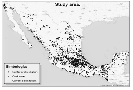Figure 1: Study area. Source: self-made.

According to [24] have increased the number of developers, industries, researchers, and other users who are making use of OSM in their applications. OSM has been compared favorably with other spatial data sources regarding spatial quality, as well as citing several examples of navigation and routing applications that make direct use of OSM data.

For this work, the cartographic base of OSM was extracted to generate the road network corresponding to the update of December 2017. Then, delimit the area of influence of each distribution center with data from Municipalities of the National Institute of Statistics and Geography (INEGI, 2017) retrieved from (http://www.inegi.org.mx) accessed on 10th June 2018; corresponding to a total of 2464 municipalities that are spatially represented by polygons. All the data has been given in shapefile format (.shp) because it is considered a standard form in the GIS environment. Figure 1 shows the area of study. Currently, the company has 11 CEDIS and 8911 active customers established throughout the Mexican Republic delimited by polygons that represent the service area of each distribution center.

For this study, we developed two scenarios solved with GIS and geospatial tools based on Location-Allocation methods. In the first scenario, we evaluated how the current allocation of customers for each distribution center is compared with a reassignment of customers with the current configuration of CEDIS; that is, customers will be assigned to their nearest distribution center.

In the second scenario, we evaluated the current allocation of customers in the same way, but we proposed the opening of four peripheral warehouses following the business plan of the company. The purpose of the opening peripheral warehouses is because the company looks for improving the service level at the same time that creates new customers. A multiple regression analysis was performed to establish which municipality has better as commercial potential and where the company does not have any CEDI.

For this regression analysis, only was considered five variables because they were the most representative at the municipality level. The variables considered are the total population, automotive vehicles registered, spare parts sales business, municipal Gross Domestic Product (GDP), and personnel employed in the industrial sector. Multiple regression was run for a total of 2464 Municipalities. Then, we took the four municipalities with the most significant potential and where the company does not have a CEDI; these are Ciudad Juarez, Tijuana, Querétaro, and San Luis Potosí. Furthermore, it was generated a midpoint within the municipality to simulate the location of the peripheral warehouses. It is applied only for this study, while in the future, to have higher precision is suggested local research of facilities. The decision will be taken according to the needs of the company. Later, to identify and analyze the coverage and distances of current CEDIS to their customers, we apply a Location-Allocation model available in ArcGIS and its extension Network Analyst tools 27 [25].

The Location-Allocation model within the GIS environment has six different types of models based on various assumptions: (1) Minimize Impedance, (2) Maximize Coverage, (3) Maximize capacitated coverage, (4) Minimize Facilities, (5) Maximize Attendance, (6) Maximize Market Share y (7) Target Market Share [26]. For this study, the first model was applied due to the nature of the problem.

3.2.  Minimize Impedance Problem

Minimize Impedance Problem attempts to find locations for a set of facilities that can minimize the sum of all weighted costs among all demands to reach the nearest facility. This type of problem is also known as P-Median that was developed by [27, 28]. In other words, the objective of the problem is to determine the appropriate locations for a specific number of facilities such that the total sum of the impedance weight can be minimized. That means that the demand is assigned to an installation multiplied by the impedance of the installation. The model has a set of constraints.

The first set of constraints is that any demand outside all impedance limits of the facilities will be considered unassigned. The second set of constraints is that for service installation has all the demands that fall within the impedance limit assigned to that installation. Finally, the last set of constraints is that the demands located within the impedance limit of more than one installation will be assigned to the nearest facility.

The problem of minimizing impedance has many applications in both the public and private sectors, including the location of retail stores, libraries, schools, hospitals, and others. Having as well as the main objective for the private sector to minimize costs and maximize efficiency, this model will reduce the total transportation costs; its use is the most appropriate for the private sector. Therefore, for the scenarios, it was decided to use this model to minimize the total distance.

3.3.  Model Formulation of P-Median

This section shows the formulation of the P-Median problem [29]:

The objective function (1) minimizes the weighted total cost. Constraint (2) means that all the demand on the demand site j must be satisfied. Constraint (3) precisely requires p facilities to be located. Constraint (4) indicates that the demand nodes can only be assigned to open facilities. Constraint (5) stipulates that the location variables must be integer and binary. Finally, the constraint (6) specifies that variable assignments be nonnegative. Bear in mind that this model does not consider the constraint of impedance, it is contained in the GIS environment.

3.4.  Methodology Summary

The first step is to design a network based on the updated OSM cartography. Once we had our network, to generate the scenario one, the Location-Allocation model was run in ArcGIS, taking the current customer’s locations and the facilities as the current CEDIS in order to have the customers assigned to the nearest CEDI minimizing the distances traveled. Scenario two was starting from the same network. The model was again run with the 11 CEDIS plus the four peripheral ones, with a total of 15 facilities and with the same demand from current customers. Here the customers were grouped by primary areas or municipalities and were located to the territories. In Figure 2, is presented a Territorial Redesign methodology.

4. Results

As a result of the first model, which consisted of the reallocation of current customers to the nearest distribution center. We observed that there was a decrease in the total kilometers traveled between the current allocation of customers from the re-allocation result. The reduction was from 1,537,814 km to 1,459,744 km, which represents an improvement of 5.08% of the distance total traveled. Only to measure it is 7.6 times the geodesic distance from Mexico City to Moscow, that is, the shortest between two points on a curved surface, as can be seen in Table 1.

In Figure 3, it can be seen that the CEDIS of Culiacán, México Norte, Mexico Sur, León, Toluca, and Villahermosa would increase their mileage, but Puebla decreases, approximately, half of the kilometers due to the re-allocation customers to other CEDIS.

Figure 4 graphically represents the proposed re-allocation for scenario one, representing a different color on the map, which would be the service area of each current distribution center.

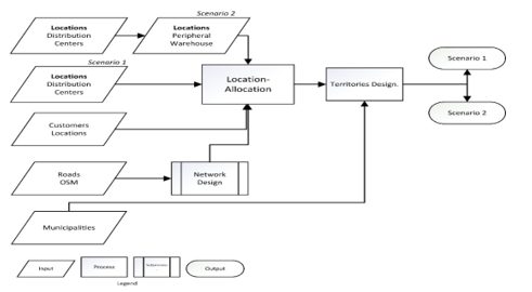Figure 2: Proposed methodology. Source: self-made.

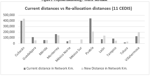Figure 3. Current distances vs. New distances for the customers’ Re-allocation (11 CEDIS). Source: self-made.

Table 1: Comparative between the current allocation and re-allocation of customers. Source: self-made.

Scenario 1
Current Allocation				Re-allocation
id	Distribution center	Current distance in Network Km	Current customers	New distance in Network Km	Re-allocated customers	%
1	Culiacán	403,064	908	436,617	969	-8.32
2	Guadalajara	111,725	887	57,120	707	48.87
3	Mérida	61,684	451	61,684	450	0
4	Monterrey	165,845	940	142,056	919	14.34
5	México Norte	39,788	1,086	57,911	1110	-45.55
6	México Sur	5,042	348	69,263	717	-1273.65
7	Puebla	441,305	2,083	212,585	1445	51.83
8	León	76,691	488	138,966	709	-81.2
9	Tampico	84,619	484	52,116	406	38.41
10	Toluca	19,882	469	36,662	539	-84.4
11	Villahermosa	128,170	767	194,763	940	-51.96
	Totals	1,537,814	8,911	1,459,744	8911	5.08

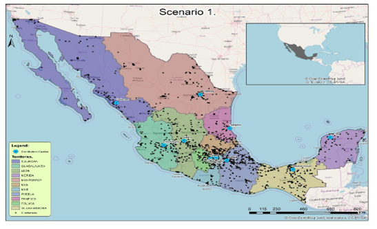Figure 4. Territorial redesign for scenario one. Source: self-made.

 For scenario two, the data was run to obtain a configuration where each current customer was re-allocated to the nearest distribution center according to the network—taking into account four peripheral warehouses that serve as auxiliary to the 11 principal CEDIS. After having solved this configuration, we obtain a reduction of 24.6% of the total trips. With this configuration, we would go from 1, 537, 814 km to 1, 159, 510 km, and there would be a reduction of 378, 304 km; it is imperative to emphasize that it is a summation of the CEDIS to each one of the customers at the national level.

With the results of this allocation, we verified that there is a significant reduction in kilometers of the CEDIS of Culiacán, Puebla, and Monterrey, which would be absorbed by Tijuana, México Sur, and Ciudad Juarez as shown in Table 2.

Table 2: Comparative results of Scenario 2. Source: self-made.

Scenario 2
		Current Distribution			Re-allocation
id	Distribution Center	Warehouse type	Current distance in Network Km	Current customers	New distances in Network Km	Re-allocated customers	%
1	Culiacán	Distribution center	403,064	908	92,085	736	77.1537523
2	Tijuana	Peripheral warehouse	0	0	79,082	148	-100
3	Guadalajara	Distribution center	111,725	887	54,962	698	50.8059969
4	Mérida	Distribution center	61,684	451	62,006	451	-0.5220154
5	San Luis Potosí	Peripheral warehouse	0	0	67,329	391	-100
6	Monterrey	Distribution center	165,845	940	89,886	836	45.8011999
7	Mexico Norte	Distribution center	39,788	1,086	51,710	1,098	-29.963808
8	Ciudad Juárez	Peripheral warehouse	0	0	35,070	79	-100
9	México Sur	Distribution center	5,042	348	69,282	648	-1274.0976
10	Querétaro	Peripheral warehouse	0	0	22,375	220	-100
11	Puebla	Distribution center	441,305	2,083	213,227	1,441	51.6826231
12	León	Distribution center	76,691	488	45,836	278	40.2328826
13	Tampico	Distribution center	84,619	484	47,247	389	44.165022
14	Toluca	Distribution center	19,882	469	33,721	552	-69.605673
15	Villahermosa	Distribution center	128,170	767	195,691	946	-52.680815
	Totals	15	1,537,814	8,911	1,159,510	8,911	24.6001142

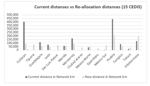Figure 5: Current distances vs. New distances for the customers’ Re-allocation (15 CEDIS). Source: self-made.

Figure 5, we can see the reductions of kilometers for Culiacan, Puebla, and Monterrey CEDIS because other CEDIS and the new proposed as peripheral warehouses like Tijuana, San Luis Potosí, Ciudad Juarez, and Querétaro now serve these customers.

As a result of the Scenario two, we can see in Figure 6, and the four other territories have been created for each new center of the peripheral distribution, as mentioned, they will be administered by another distribution center to cover the demand of the customers assigned to these territories.

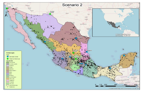Figure 6. Territorial redesign of scenario 2. Source: self-made.

Discussion and Conclusion

Comparing the two scenarios, we can discuss that for Scenario one; there is a decrease of 5.08 % concerning the total distance. In the same way, the company will obtain a reduction in the costs of transport and raise the service level. For Scenario 2, where the 11 current CEDIS and four peripherals warehouses are considered. Likewise, there is a reduction in mileage of 24.6%. This configuration would have higher coverage to customers and lower transportation costs, but this would depend on the number of the peripheral warehouses opened. This scenario must be made an economic evaluation due to the investment that entails the opening of new facilities. The value of this work is to be taking into account real-world results and manage a large amount of data as well as consider the constraint of impedance. The continuation of this study will be compared to the operating cost of the peripheral warehouse and the variations of income for each CEDI.

In conclusion, establishing four peripheral warehouses, the routes that were considered foreign and thus more expensive because the route has a long time to arrive with the customers, now are considered as local routes. With this proposal, the local routes guarantee the delivery in a maximum 3 hours instead of 24 to 36 hours. Moreover, the proposal generates the plus of being able to attract more customers in the new territories and always improving the service level to the customers.

Conflict of Interest

The authors declare no conflict of interest.

Acknowledgment

The corresponding author wants to acknowledge financial support from Consejo Nacional de Ciencia y Tecnología (CONACyT) with the number of scholarships (391444) and the Popular Autonomous University of the State of Puebla (UPAEP University).

1.  G. Ghiani, G. Laporte, R. Musmanno, Introduction to Logistics Systems Management, Wiley, 2013.
2.  C. Lo, A. Yeung, Concepts and Techniques in Geographic Information Systems, Pearson Prentice Hall, 2007.
3.  R. Church, A. Murray, Business Site Selection, Location Analysis, and GIS, Wiley, 2009.
4.  R. Church, “Location modelling and GIS.” In: P. Longley, M. Goodchild, D. Maguire, D. Rhind, Geographical information systems, 293-303, Wiley, 1999.
5.  R. Church, “Geographic information systems and location science” Comput Oper Res, 29, 541–562, 2002.
6.  B. Alhenaki, “Using GIS/GPS to Optimize Supply Chain Management and Logistics at Walmart” International Journal of Scientific & Engineering Research, 7, 745-748, 2016.
7.  X. Li, A. Gar-On, “Integration of genetic algorithms and GIS for optimal location search” International Journal of Geographical Information Science, 19, 581-601, 2005.
8.  M. Delivand, A. Cammerino, P. Garofalo, M. Monteleone, “Optimal locations of bioenergy facilities, biomass spatial availability, logistics costs, and GHG (greenhouse gas) emissions: a case study on electricity productions in South Italy” Journal of Cleaner Production, 99,129-139, 2015.
9.  L. Gigovic, D. Pamucar, Z. Bajic, M. Milicevic, “The Combination of Expert Judgment and GIS-MAIRCA Analysis for the Selection of Sites for Ammunition Depots” Sustainability, 8, 1-30, 2016.
10.  F. Zhang, J. Wang, S. Liu, S. Zhang, J. Sutherland, ” Integrating GIS with an optimization method for a biofuel feedstock supply chain, Biomass and Bioenergy, 98, 194-205, 2017.
11.  K. Sahoo, G. Hawkins, X. Yao, “GIS-based biomass assessment and supply logistics system for a sustainable biorefinery: A case study with cotton stalks in the Southeastern US” Applied Energy, 182, 260-273, 2016.
12.  J. Irizarry, E. Karan, F. Jalaei, “Integrating BIM and GIS to improve the visual monitoring of construction supply chain management” Automation in Construction, 31, 241–254, 2013.
13.  Z. Ma, Y. Ren, “Integrated Application of BIM and GIS: An Overview” Procedia Engineering, 196, 1072 – 1079, 2017.
14.  A. Susanty, D. Sari, W. Budiawan, Sriyanto, H. Kurniawan, “Improving green supply chain management in the furniture industry through Internet-based Geographical Information System for connecting the producer of wood waste with the buyer” Procedia Computer Science, 83, 734–741,2016.
15.  F. Zhang, D. Johnson, M. Johnson, D. Watkins, R. Froese, J. Wang, “Decision support system is integrating GIS with simulation and optimization for a biofuel supply chain” Renewable Energy, 85, 740-748, 2016.
16.  G. Buzai, “Location-allocation models applied to urban public services Spatial analysis of Primary Health Care Centers in the city of Luján, Argentina” Hungarian Geographical Bulletin, 62, 387-408, 2013.
17.  V. Dumbliauskas, V. Grigonis, A. Barauskas, “Application of Google-based data for travel time analysis: Kaunas City case study” Promet-Traffic & Transportation, 29, 613-621, 2017.
18.  F. Wang, Y. Xu, “Estimating O-D Travel Time Matrix by Google Maps API: Implementation, Advantages, and Implications” Annals of GIS, 17(4), 199-209, 2011.
19.  S. Sehra, J. Singh, R. Singh, “Assessing OpenStreetMap Data Using Intrinsic Quality Indicators: An Extension to the QGIS Processing Toolbox” Future Internet, 9, 1-22, 2017.
20.  E. Olivares-Benitez, P.N. Ibarra, S. Nucamendi-Guillén, O.G. Rojas, “Multi-Objective Territory Design for Sales Managers of a Direct Sales Company.” In Optimizing Current Strategies and Applications in Industrial Engineering, 160-178, IGI Global, 2019.
21.  L. Hervert-Escobar, V. Alexandrov, “Territorial design optimization for business sales plan” Journal of Computational and Applied Mathematics, 340, 501-507, 2018, https://doi.org/10.1016/j.cam.2018.02.010
22.  E. Burkholder, “Spatial Data, Coordinate Systems, and the Science of Measurement” Journal of Surveying Engineering, 127, 143-156, 2001.
23.  J. Arsanjani, A. Zipf, P. Mooney, M. Helbich, “An introduction to OpenStreetMap in Geographic Information Science: Experiences, research, and applications.” In: A. Jokar, A. Zipf, P. Mooney, M. Helbich, Eds. OpenStreetMap in GIScience, Lecture Notes in Geoinformation and Cartography, 1–18, Springer International Publishing Switzerland, 2015.
24.  P. Mooney, M. Minghini, “A Review of OpenStreetMap Data. In: Foody G. See L. Fritz S. Mooney P. Olteanu-Raimond A. Fonte C. and Antoniou V” Eds. Mapping and the Citizen Sensor, 37–59, London: Ubiquity Press, 2017.
25.  ESRI 2011. ArcGIS Desktop: Release 10. Redlands, CA: Environmental Systems Research Institute.
26.  ESRI 2018. Location-allocation analysis-Help | ArcGIS Desktop, Desktop.arcgis.com, Retrieved from http://desktop.arcgis.com/en/arcmap/latest/extensions/networkanalyst/locationallocation.htm#ESRI_SECTION1_F8182D9F421E4EA4AEE11E7B360E1340 (accessed on 10th May 2018).
27.  S. Hakimi, “Optimum location of switching centers and the absolute centers and medians of a graph” Oper Res, 12, 450–459, 1964.
28. S. Hakimi, “Optimum distribution of switching centers in a communication network and some related graph-theoretic problems” Oper Res, 13, 462–475, 1965.
29.  G. Laporte, S. Nickel, F. Saldanha da Gama, Location Science, Springer, 2015.

(Click Here)

(Click Here)