1 Introduction

The analysis of employment processes and estimation of factors that affect job tenure is frequently made by using survival analysis. Several authors have studied the effect that wages have on staying at work using microeconomic data [1,2]. Gregory-Smith and Thompson [3] have inspected the job tenure of CEOs in the United Kingdom and their exit using survival analysis. Jackowska and Wycinka [4] have made an assessment of the last period of employment for unemployed persons. Kohara, Sasaki, and Machikita [5] present that job tenure is an evidence of a job full of quality after unemployment. Grzenda and Buczyński [6] have assessed the employee turnover using competing risks models. Chaudhuri, Reilly, and Spencer [7] examine the effects of age and tenure on job satisfaction. Altunbaş, Thornton and Uymazc [8] analyze if there is a link between job tenure of an employee and misconduct by US banks. Worker aging has affected in the job tenure distribution. Also, a shift toward longer-duration jobs is because of the declining business [9, 10, 11].

Sometimes, for employees, job tenure is an important criterion in starting new job, and for employers when they have to hire new employees. When the time of staying in employment relationship with the same employer and the same job position is too long (more than 5 years), the worker has the advantages of being considered a loyal employee.

But on the other hand, employees may become less motivated [12, 13]. When the time of staying in employment relationship with the same employer and the same job position is very short (less than 2 years), the employees have the opportunity to gain more experience working in different job positions and with different people.

Survey reports by Wolfe [14] have shown that the average job tenure for employees is around 7 years. From the results, fifth of workers have been in the same company and in the same job position for more than ten years, while more than a third of them stay for 5-10 years.

Bureau of Labor Statistics [15], for year 2018, have shown that older employees have a median job tenure higher compared with the median time for younger ones. If an employee is 55 to 64 years old, the median job tenure is around ten years, while for an employee ages 25 to 34, this time is 2.8 years. Older employees have been in the same job for ten years or more, while younger employees are more likely to have short job tenure. In January 2018, 74 percent of employees from 16 to 19 years old have been in a current job for one year or less. Only 12 percent of employees ages 30 to 34 had job tenure for 10 years or more, where for employees between 60 to 64 years old, more than half of them had this job tenure.

In this study, we have examined of the characteristics of 887 employees, in several different private and public companies, in Albania. We will adopt Kaplan-Meier method [16], and the Cox proportional hazards model [17], in modeling the duration of job tenure. Our data are right censuring because some employees are still in the same company and in the same job position by the end of the sample.

In addition to the survival time, job tenure and indicator variable, we have taken into consideration also other variables that are thought of as important factors in the job tenure. The factors studied are the current age of the employee, the age at which he started the job, salary, gender, position, education, marital status and years of work in front of the current position. This study determine the factors which affect the job tenure using Cox proportional hazards model.

The analysis is done through R software, using survival() coxphMIC() and ggplot2() packages.

2. Materials and methods.

2.1.  Cox proportional hazards (Cox PH) model

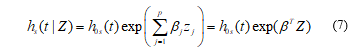
The Survival analysis models the timing of events by using statistical methods. Cox proportional hazards model is a regression model for the survival data, which analysis the relationship between covariates and survival [18]. This model has been proposed by Cox, 1972, [17] and the hazard function relates with covariates as follows

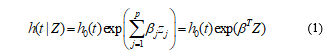where  is the vector of covariates for a particular individual,  is a parameter vector of regression coefficients and  is the baseline hazard function. This function is the hazard function when all covariates are ignored and shows how the risk changes with time. Factors effect on the hazard function in a multiplicative way and the baseline hazard function stay an unspecified and nonnegative function of time, even with the addition of explanatory covariates.

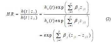
In the Cox PH model, the ratio of hazard functions for different individuals does not depend on time. For two individuals with covariate values  and , the hazard ratio [17] is:

2.2.  Maximum Partial Likelihood Estimate

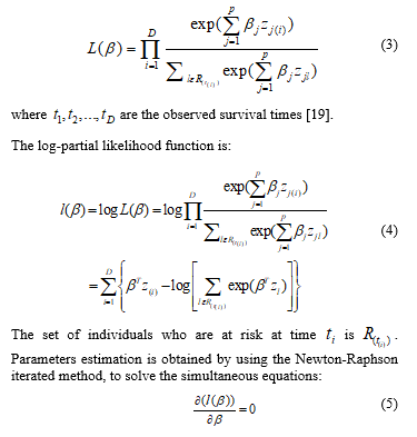
In regression models, the most common method for parameter estimation is the maximum likelihood method. To use the likelihood function, we should know the distribution of the data. However, one of the main features of the Cox model is that the baseline hazard function is not identified parametrically. Therefore, the ordinary likelihood function cannot be used for the Cox PH model. As an alternative, a method called Maximum Partial Likelihood Method has been proposed by Cox.

Sufficient conditions for the estimation of the maximum partial likelihood function, when there are missing at random variables data, have been provided by Chen, Ibrahim and Shao [19]. They also provide necessary conditions in the case of no missing data.

The partial likelihood function is:

2.3.  Adequacy assessment of the proportional hazards model

The next step after selecting the model, is to evaluate the assumption of proportionality and the goodness of fit, thus we evaluate the fitted model. In order to verify the proportional hazard assumption, there are graphical methods, statistical tests, and time-dependent variables. There are different types of residuals for a proportional hazard model such as: Cox-Snell residuals [20], Schoenfeld residuals by Schoenfeld [21], deviance residuals [22] and dbeta residuals.

Schoenfeld residuals [21] are given by

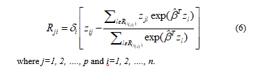This method was modified by Grambsch and Therneau [23]. These residuals are good estimators if we want to check for the time trend or for the lack of proportional hazards assumption, because they have the same properties as random walk. A non-zero slope shows that the proportional hazard model is not valid, because the conditions of proportionality are not met. Except graphical methods, Schoenfeld has proposed a global goodness-of-fit test.

2.4.  Stratified proportional hazards model

The assumption of proportional hazards model may not always be met in practical situations. To accommodate the non-proportional hazards cases, Cox model can be modified using the concept of stratification for the covariate that does not satisfy the proportionality. This model has the form:

where  for k strata and are s unknown baseline hazard functions [24].

By using stratification we get different baseline hazard functions for each stratum, but the coefficients of the variables taken into consideration are ordinary across strata. In a stratified Cox proportional hazards model, the assumptions of proportionality hold within each stratum, but it does not necessarily hold for the combined data. There are also special cases when the effect of the factor differs within strata [24].

2.5.  Minimizing approximated Information Criteria

The vector of regression coefficients can be estimated by maximizing the partial log-likelihood [17]. To indicate the zero elements in  and the nonzero ones, we have to look for methods obtained from penalized partial likelihood function. Selection of important covariates in survival analysis is possible by using best subset selection (BSS) algorithm or the regularization one.

Su, Wijayasinghe, Fan, and Zhang [25] elaborated Minimizing Approximated Information Criteria (MIC) method to handle sparse estimation of Cox PH models. This model enjoys the advantages of best subset selection (BSS) algorithm and the regularization one.

3. Study population

In our analysis we have analyzed job tenure for 887 employees, in Albania. Job tenure is the time that employees have been in their current job or with their current employer. The analysis is based on samples taken from the database of employees, in several different private and public companies.

The study period is January 1991 – December 2018. The start time is the time when the employee begins the financial relationship with the employer. End time is the time of interruption of financial relations. The job tenure time is month.

A major problem encountered when analyzing survival data is that of censored data. In this study, censored data refers to those employees who were still working at the time when the data was last updated. In this study, with time, we refer to the job tenure in months and the survival function gives the probability that the employee will stay in a working relationship for a certain time.

On the other hand, the hazard function gives us the potential risk that the employee will terminate the relationship with the company after a certain time.

In addition to the survival time, time from the beginning of the relationship with the company, until the end of the term and the indicator variable, whether or not an employee is still working, we have taken into consideration also other variables that are thought of as important factors in the job tenure. The factors studied are the current age of the employee, the age at which he/she started the job, salary, gender (male, female), position (engineer, supervisory, specialist, financier and other positions(driver, cleaner, babysitter, etc.)), education (middle school, high school and university), marital status (married, unmarried) and years of work in front of the current position.

4. Results

Among the 887 employees, 534 of them (60%) were still in work in December 2018, and 353 of them (40%) had interrupted the employment relationship with the company. The average job tenure for employees who are not in work, is around 4 years, 35% of the workers have been in the same job position, with the same employer, for more than 8 years.

If we consider the job tenure for employees still at work, together with the job tenure for the employees how are not at work, we see that 26 % of the workers have been in the same company and in the same job position, for more than 10 years and 30% of them for less than 2 years.

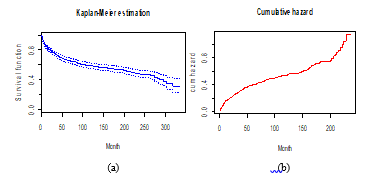Figure 1: Estimated survival function (a) and cumulative hazard function (b), for job tenure.

Figure 1 shows that the probability of job tenure in the first year since the start of the work reaches 84.6%. The minimum period of time spent in a current job is one month and the maximum time is 317 months, approximately 26 years.

The first quartile of job tenure is 33 months; in other words, 25% of employees interrupt their relationship with the company within 33 months from their beginning. The possibility of extending the job tenure at least 217 months from the start is 50%.

Also, we have made a gender-related comparison to evaluate whether there is any difference in job tenure between them. From the studied data, we have that, 29% are women and 71% are male.

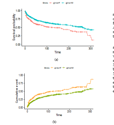Figure 2: Kaplan-Meier estimation curves (a) and cumulative hazard (b) for male and female

Figure 2 shows that for men the estimated survival curve lies above the survival curve for women. This is as a result of the fact that job tenure for men is greater than that for women. Half of the men will interrupt employment relationships within 262 months, while women within 121 months. The probability of staying in relationship with the company in the first year is 87% for males and 78.5% for females. The first quartile of job tenure is 42 months, 25% of men will leave the company within 42 months, while women within 17 months.

To study whether the two Kaplan-Meier curves for gender are statistically equivalent, statistical tests (log-rank test, Gehan-Wilcoxon test and Peto-Peto test) have been used. From their results there is a statistically significant difference between Kaplan-Meier curves for women and that for men, with a critical value almost zero. The inhibiting effect young children have on the work lives of wives may help account for differences in job tenure by marital status. To assess whether there is a difference in job tenure between married and unmarried employees, we have used survival curves.

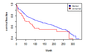Figure 3: Kaplan-Meier estimation curves for married and unmarried employees

Figure 3 shows that the survival curve for married employees, measured by the Kaplan-Meier method, lays above the survival curve for the unmarried employees, which mean that the job tenure for married employees is greater than that of unmarried employees. At a time of 150 months of work, 75% of married employees are still at work, while only 50% of the unmarried will be in work at this time.

We have used the Cox proportional hazard model, in order to assess the impact of the factors in job tenure, as a semi-parametric model for the survival analysis. Initially, we have built dummy variables for actual age, age at the beginning of the job and the salary. The variables are: ageA = 1 if the employee is between 20-30 years old and = 0 otherwise, ageB = 1 if the employee is between 30-50 years old and = 0 otherwise, if one employee is over 50 years old than ageA = 0 and ageB = 0. The same is done with the age at the beginning of the job. For the salary: salA = 1 if the employee has a salary up to 40,000 and = 0 otherwise, salB = 1 if the employee has a salary 40,000-70,000 and = 0 otherwise, if one employee has a salary greater than 70,000, salA = 0 and salB = 0.

Table 1: Cox proportional hazard analysis

Variable	coef	exp(coef)	Pr(>|z|)
Ywcp	-0.0043	0.9957	0.0000***
genderM	-0.3622	0.6961	0.020*
maritalstMarried	-0.13	0.8932	0.4959
educMiddle	1.1520	3.1650	0.0453
educUniversity	0.3051	1.357	0.5631
posEngineer	-0.0439	0.9570	0.8324
posSupervisory	-2.354	0.0950	0.0000***
posOther	-1.1450	0.3182	0.0000***
posSpecialist	-1.4420	0.2366	0.0000***
ageA	1.2740	3.5750	0.0005***
ageB	1.1020	3.0110	0.0000***
agebiA	-2.6150	0.0732	0.0000***
agebiB	-1.5440	0.2136	0.0000***
salA	-2.8370	0.0586	0.0083**
salB	-0.2013	0.8177	0.1869
Likelihood ratio test= 373.3 on 15 df,  p=<2e-16 Wald test          = 234.7  on 15 df,   p=<2e-1

where: ywcp-years of work in front of the current position; genderM-gender (male); maritalstMarried- marital status (married); educMiddle- education (middle school); educUniversity- education (university); posEngineer-position (engineer); posSupervisory-position (supervisory); posSpecialist-position(specialist); posOther-other positions (driver, cleaner, babysitter, etc.); ageA-employee age 20-30; ageB-employee age 30-50; ageA- age at the beginning of the job 20-30; ageB- age at the beginning of the job 30-50; salA- salary up to 40,000; salB- salary 40,000-7000;

The variables are rated as significant using a 0.05 level. The results are obtained from survival() package, in R statistical software.

Table 2: Final Cox proportional hazard model

Variable	coef	exp(coef)	Pr(>|z|)
ywcp	-0.0040	0.9960	0.0000
genderM	-0.3622	0.6961	0.020
posEngineer	-0.6097	0.5435	0.0000
posSupervisory	-2.0140	0.1334	0.0000
posOther	-1.5470	0.2130	0.0000
posSpecialist	-1.5940	0.2030	0.0000
ageA	1.5800	4.8530	0.0000
ageB	1.1690	3.2180	0.0000
agebiA	-2.3820	0.0923	0.0000
agebiB	-1.3950	0.2478	0.0000
salA	-2.6340	0.0718	0.0095
salB	-0.4061	0.6662	0.0063
Concordance= 0.813 (se = 0.013 ) Likelihood ratio test= 339.4 on 12 df,  p=<2e-16 Wald test            = 220.4  on 12 df,   p=<2e-16 Score (logrank) test = 374.3  on 12 df,   p=<2e-16

The first column of the table shows the parameters estimation, with the partial likelihood method. The second column shows the hazard ratio. According to the Cox PH analysis, variables: actual age, age at the beginning, salary, gender, time of work before the current job (ywcp) and position in the company are significant variables with a p-value which is less than 0.05. The marital status variable and education are not targeted as important factor. We can observe this from p-values and also from confidence intervals of hazard ratio which contain the null value of one.

Based on the results of Table 1, we perform Cox PH multivariate model using the stepwise selection method with all the variables that have a p-value of less than or equal to 0.05. These results are presented in the following table, which also presents the final model.

The Cox proportional hazard model of our data, based on table 2, referred to the theoretical Cox model, equation 1, is given by:

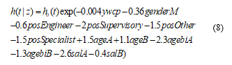From this model we can conclude that the greater the age at the moment of the beginning of the job, the higher the salary and the greater the number of years in work before this job, the possibility of dismissal is smaller. The position and the gender affect negatively in the interruption of the relationship between the employee and the company, while the age, affect positively in dismissal.

If we keep the other variables constant, the estimated risk of dismissal for an employee, with age less than 30 years is approximately equal to exp(1.58)=4.853 times higher than an employee with age greater than 50 years old. Employees between 30 years old to 50 years old at the time they start the job have 75% less risk of being dismissed than an employee over 50 years old at the moment he/she begin the job.

If we assumed that two employees are of the same gender, have one job position, belong to the same age category, the hazard ratio for an employee with salary between 40,000 to 70,000, compared to an employee with a salary fewer than 40,000, is 9.28. So, employees with a salary between 40,000 to 70,000 have 9.28 fewer risks to be dismissed, compared to employees with a salary fewer than 40,000.

Table 3: Model checking using Schoenfeld residuals.

	rho	chisq	p
Ywcp	0.0055	0.0110	0.9163
genderM	0.0588	1.1500	0.2845
posFinancier	-0.0696	1.4100	0.2346
posOther	0.0338	0.3540	0.5520
posSpecialist	-0.0032	0.0028	0.9579
posSupervisory	-0.1436	0.0000	0.9999
ageA	-0.0187	0.0846	0.7712
ageB	-0.0879	1.7000	0.1923
agebiA	-0.0233	0.1340	0.7147
agebiB	-0.0115	0.0332	0.8554
salA	0.0347	0.2980	0.5853
salB	-0.1975	13.700	0.0002
GLOBAL	NA	25.400	0.0129

For a male, the risk of being dismissed is reduced by 30% compared to a female. If the job position of an employee is an engineer, this reduces the risk of leaving with 45% compared to a financier. The likelihood-ratio tests, Wald test and the score test in this case, show that the underlying hypothesis, the assumption that all the coefficients are zero, is rejected.

The next step after selecting the model, is to evaluate the assumption of proportionality. We have used Schoenfeld residuals to evaluate if the variables taken into account in the model meet the requirements of the proportional hazard.

From Table 3 it is clear that the variable salB does not meet the PH conditions with a p-value less than 0.05. Also, the global test is not quite statistically significant.

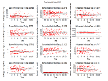Figure 4: Schoenfeld residuals

Figure 4 shows the plot of Schoenfeld residuals for actual age, age at the beginning, salary, gender, time of work before the current job and position in the company versus survival time (job tenure). Slope of the fitted linear regression line for variable salB is different from zero, because the p-value is 0.002<0.5. Salary violates the assumption of proportionality; thus we can conclude that this variable may depend on time.

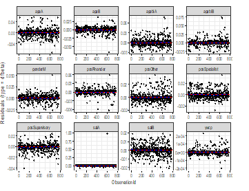Figure 5: Graph of dfbeta indexes for the Cox model.

Slopes taken from the fitted linear regression lines for actual age, age at the beginning, gender, time of work before the current job and position are not significantly different from zero, since their p-values are greater than 0.05.

We have visualized the dfbeta values, for each covariate, to test outliers. These plots, given in figure 5, show the estimated differences in the regression coefficients and the magnitudes of the largest dfbeta.

For some variables the dfbeta indexes have a greater value then the others. But the above index plots show that none of the sample affects individually.

From the plots of Schoenfeld residuals we concluded that the variable salary does not meet the assumption of proportionality. One way to deal with this is by using the stratified Cox regression model. The results of the new model are given in Table 4.

Table 4: Results for the stratified Cox model

	coef	exp(coef)	Pr(>|z|)
ywcp	-0.0037	0.9963	0.0000
genderM	-0.4507	0.6371	0.0003
posEngineer	-0.6097	0.5435	0.0000
posSupervisory	-2.2815	0.1021	0.0000
posOther	-1.5090	0.2211	0.0000
posSpecialist	-1.5290	0.2167	0.0000
ageA	1.6050	4.9770	0.0000
ageB	1.2500	3.4920	0.0000
agebiA	-2.3500	0.0954	0.0000
agebiB	-1.4370	0.2376	0.0000

Table 4 shows that all the variables are statistically significant after stratification.

Also, Schoenfeld residuals given in Table 5 show that all variables meet the PH assumption.

Table 5. Testing the PH assumption by using Schoenfeld residuals, for the stratified model.

	rho	chisq	p
Ywcp	0.0269	0.2690	0.6042
genderM	0.1037	3.5700	0.0587
posEngineer	0.0865	2.1800	0.1394
posSupervisory	-0.0685	0.0000	0.9999
posOther	0.0999	2.8700	0.0900
posSpecialist	0.1117	3.3800	0.0658
ageA	-0.0030	0.0021	0.9635
ageB	-0.0385	0.3550	0.5515
agebiA	-0.0300	0.2180	0.6402
agebiB	-0.0322	0.2660	0.6063
GLOBAL		14.2000	0.2234

Also from Table 5 we can see that the global test is quite statistically significant.

Additionally, the MIC (minimizing approximated information criteria) method was used in the selection of variables. The results are given in Table 6 and are taken with the R package coxphMIC [26].

MIC started with maximum partial likelihood method given by the first column. From the last two columns of the table we get the estimates for the coefficients, which show that the selected variables are the same as those selected by the Cox PH method.

	beta0	p.value	beta.MIC	se.beta.MIC
Gender	0.1439	0.0058	0.1476	0.0527
Position	-0.5434	0.0000	-0.5432	0.0530
ageA	0.7430	0.0000	0.7487	0.0976
ageB	0.6205	0.0000	0.6236	0.0828
agebiA	-0.8385	0.0000	-0.8457	0.1294
agebiB	-0.5442	0.0000	-0.5489	0.1049
salA	0.4442	0.0000	0.4560	0.0478
salB	-0.0251	1.0000	0.0000	NA

Table 6: Variable selection with MIC method.

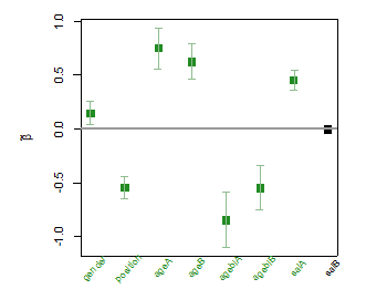Figure 6: Error bar plot for MIC estimates of gamma and beta, together with the 95% confidence intervals. The selected variables are highlighted in green.

Figure 6 presents variables which are statistically significant with the MIC method. The selected variables are green in color, and are also associated with their confidence intervals. We can see that variable salB is not considered as significant covariates. The first plot is the error bar plot for estimators.

5. Conclusion

In this study, we have examined of the characteristics of 887 employees, in several different private and public companies, in Albania. We have used the Cox PH model in order to assess the impact of the factors in job tenure. According to the Cox PH analysis, variables: actual age, age at the beginning, salary, gender, time of work before the current job and position in the company are statistically significant, while the status variable and education are not targeted as important factor.

The findings of the present study showed that the average job tenure of an employee on a given company is approximately 187 months, different from the results taken by Wolfe [14].

Among employees, 26 % of them have been in the same company and in the same job position, for more than 10 years and 30% of them for less than 2 years. Job tenure for men is greater than that for women.

Young workers have the lowest levels of job tenure. Employees aged between 30 to 50 years at the time they start the job have 75% less risk of being dismissed than an employee over 50 years old at the moment he begin the job. Employees with a salary between 40,000 to 70,000 have 9.28 fewer risks to be dismissed, compared to employees with a salary fewer than 40,000. Men have higher overall median levels of tenure than women, their risk of being dismissed is reduced by 30% compared to a female.

1. J. Kettunen. Effects of wages on job tenure. Journal of income distribution. Volume 9, Issue 2, Pages 155-169. (2000) https://doi.org/10.1016/S0926-6437(00)00011-1
2.  L. Munasinghe, T. Reif, A. Henriques. Gender gap in wage returns to job tenure and experience. Labour Economics, Volume 15, Issue Pages 1296-1316. (2008) https://doi.org/10.1016/j.labeco.2007.12.003.
3.  I. Gregory-Smith, S. Thompson, P.W. Wright. Fired or Retired? A Competing Risks Analysis of Chief Executive Turnover. (2009)
4.  B. Jackowska, E. Wycinka. Analysis of the last employment period of the unemployed: the application of the Cox model. Folia economica 255. (2011)
5.  M. Kohara, M. Sasaki, T. Machikita. Is longer unemployment rewarded with longer job tenure? Journal of the Japanese and International Economies. Volume 29, Pages 44-56. (2013) https://doi.org/10.1016/j.jjie.2013.06.002
6.  W. Grzenda, M. Buczyński. Estimation of employee turnover with competing risks models. Folia Oeconomica Stetinensia. (2015) DOI: 10.1515/foli-2015-0035.
7.  K. Chaudhuri, K. Reilly, D. Spencer. Job satisfaction, age and tenure: A generalized dynamic random effects model. Econimics letters. (2015) https://doi.org/10.1016/j.econlet.2015.02.017
8. Y. Altunbaş, J. Thornton, Y. Uymazc. CEO tenure and corporate misconduct: Evidence from US banks. Finance Research Letters, Volume 26, Pages 1-8. (2018) https://doi.org/10.1016/j.frl.2017.11.003
9. J.P. Hausknecht, C. Trevor. Collective turnover at the group, unit, and organizational levels: Evidence, issues, and implications. Journal of Management, 37 (1), pp. 352-388. (2011)
10. H. Hyatt, J. Spletzer. The shifting job tenure distribution. Labour Economics. (2016) https://doi.org/10.1016/j.labeco.2016.05.008
11.  J. Son, Ch. Ok. Hangover follows extroverts: Extraversion as a moderator in the curvilinear relationship between newcomers’ organizational tenure and job satisfaction. (2019) https://doi.org/10.1016/j.jvb.2018.11.002
12.  T. Ng, D. Feldman. Does longer job tenure help or hinder job performance? Journal of Vocational Behavior. Volume 83, Issue 3. (2013) https://doi.org/10.1016/j.jvb.2013.06.012
13.  C Chen, Y. Kao. Moderating effects of work engagement and job tenure on burnout–performance among flight attendants. Journal of Air Transport Management. Volume 25, Pages 61-63. (2012) https://doi.org/10.1016/j.jairtraman.2012.08.009
14. P. Wolfe. Trends in Job Tenure—and What Employers Should Do About Them. (2017) http://blog.indeed.com/2017/06/29/trends-job-tenure/
15.  Bureau of Labor Statistics. “About the U.S. Bureau of Labor Statistics” Accessed Oct. 14, 2019.
16. E. Kaplan, P. Meier. Nonparametric estimation from incomplete observations. Journal of the American Statistical Association, vol. 53, pp. 457–481. (1958)
17.  D.R. Cox. Regression models and life tables, Journal of the Royal Statistical Society B, 34, 187-202. (1972).
18.  T. Themeau, P. Grambsch. Modeling Survival Data: Extending the Cox Model, New York: SpringerVerlag. (2000).
19.  M. Chen, J. Ibrahim, Q. Shao. Maximum likelihood inference for the Cox regression model with applications to missing covariates. Journal of Multivariate Analysis. (2009). https://doi.org/10.1016/j.jmva.2009.03.013
20.  D. R. Cox, E.J. Snell. A general definition of residuals (with discussion). Journal of the Royal Statistical Society, Series B 30:248-275. 5. (1968).
21.  D. Schoenfeld D. Partial residuals for the proportional hazards regression model. Biometrika 69(1):239-241. (1982).
22.  T.M. Therneau, P.M. Grambsch, T.R. Fleming. Martingale-Based Residuals and Survival Models. Biometrika, 77, 147—160. (1990).
23.  P.M. Grambsch, T.M. Therneau. Proportional Hazards Tests in Diagnostics Based on Weighted Residuals. Biometrika, 81, 515—526. (1994).
24.  L. Thompson, R. Chhikara, J. Conkin. Cox Proportional Hazards Models for Modeling the Time To Onset of Decompression Sickness in Hypobaric Environments. NASA/TP–2003–210791. (2003).
25.  X. Su X, C. S. Wijayasinghe, J. Fan, Y. Zhang. Sparse estimation of cox proportional hazards models via approximated information criteria. Biometrics, 72:751–759 (2016).
26.  R. Nabi, X. Su X. coxphMIC: An R package for sparse estimation of Cox proportional hazards models via approximated information criteria. Ar.Xiv:1606.07868v2. (2017)

(Click Here)

(Click Here)