1. Introduction

This paper is an extension of the work originally presented in CSCS22: The 22^nd International Conference on Control Systems and Computer Science, Bucharest, 2019 [1].

Worldwide, air pollution has extensive effects on the environment, human health and global economy, as research showed correlation between premature deaths and low air quality [2,3]. The extent of the consequences of air pollution levels are strongly related to the pollutant concentrations and the level of exposure. Until recently, the assessment of air quality has been strongly reliant on traditional monitoring networks, because of their accuracy, but they also have some disadvantages that should not be disregarded [4,5]. The main issues of these monitoring networks are high costs of acquisition, maintenance requirements, improper placement in areas with low pollution and the limited number of fixed stations, due to legal restrictions for location [6]. Therefore, the need for alternative air pollution measurements is indisputable, in the context of spatial variability of air quality [7-9]. As a result of the variety of sensors on the market, the increased computing power and new communication protocols and the community-led sensing initiative, the topic of air pollution became a key research topic, at local and regional scale [10].

The research community expressed concerns particularly regarding the dangerous effects on human health of two key pollutants: nitrogen dioxide and particulate matter (PM). The latter is one of the most dangerous pollutants in terms of health effects, as it can cause a wide range of negative reactions, even at low concentrations [11]. Among them, the PM₁₀ (PM with diameter lower than 10 µm) and PM_2.5 (PM with diameter lower than 2.5 µm) are considered to have the greatest impact, as their effects are not only related to pollutant concentrations, but also to the frequency and the duration of exposure [12]. For individuals, there are also other factors that play important roles in the extent of air pollution effects, such as health status and age [13].

The prime sources of particulate matter in the atmosphere are either natural, such as volcano eruptions and forest fires, or human-made, such as traffic, industry, agriculture, construction and other combustion processes. PM concentrations are particularly important to monitor due to the fact that they can be emitted not only from direct emission sources, but also from chemical reactions between different gases, such as NOx and SO2 [14]. A comprehensive characterization of PM has to consider multiple factors: (1) mass; (2) elemental composition; (3) water-soluble ionic species; and (4) organic compounds. The traditional sampling systems based on gravimetric measurements of collected particles generate direct measurements of airborne particle mass. Moreover, during the sampling process, there is the possibility of losing the semi-volatile organic compounds and semi-volatile ammonium compounds (such as NH₄NO₃). The composition of the sample of PM is also decisive for the accuracy of the measurements, because the presence of ionic species (i.e. sulfate and nitrate compounds) increases the liquid water uptake of suspended particles and therefore, the particle dimension. Therefore, the chemical composition of the sample and the temperature heavily influence the correct assessment of PM concentrations in the atmosphere [15].

This paper presents an analysis of the variation of particulate matter (PM10 and PM2.5) concentrations in relation to relative humidity. Chapter 2 compiles related work for data accuracy of PMs, Chapter 3 discusses the method that it is used, Chapter 4 presents the results, and lastly, Chapter 5 concludes the paper.

2. Related Work

The effects of different parameters on the data accuracy of PM concentrations were approached in several papers. The influence of wind and precipitation on different-sized particulate matter concentrations were investigated in paper [16], showing that the effects of atmospheric conditions differ, depending on the size of the particulate matter.  The increase in wind speed can decrease the concentrations of fine PM, while decreasing the concentrations of coarse PMs. The authors also found a stronger negative impact of precipitation on PM₁₀ than on PM_2.5.

In paper [17], authors analyze the way PM₁₀ concentrations are influenced by different meteorological parameters, such as pressure, relative humidity, temperature, wind speed, wind direction, CO, SO₂, NO, NO₂. A quantile regression model has been employed and the results showed that the influence of the independent variables was significant in at least one or more quantiles of the PM₁₀ concentrations. Among the analyzed parameters, relative humidity was proven to have a significant impact on quantiles 0.05 to 0.3 and an insignificant impact at higher quantiles.

The topic of the relationship between relative humidity and PM concentrations was approached in paper [18]. Authors found that PM concentrations in the atmosphere are closely correlated with the levels of relative humidity. It has been shown that high humidity conditions (between 70-100%) led to a reduction in PM_2.5 concentrations, while low-humidity conditions (below 70%), led to the increase in PM_2.5 concentrations. In case of PM₁₀ concentrations, humidity values below 45% had an accumulation effect, causing an increase in concentration, while an environment with humidity levels above 45% led to lower concentrations.

3. Methods

3.1.  Tel-MonAer platform

The aim of the Tel-MonAer project was the development of a mobile, extensible and scalable system which integrates technologies such as the Internet of Things and Edge/Cloud Computing, for the purpose of monitoring and performing real time analysis of the risk factors of public health and the environment. The architecture of the IoT platform is presented in Figure 1.

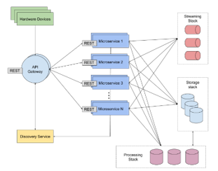Figure 1: NETIoT architecture

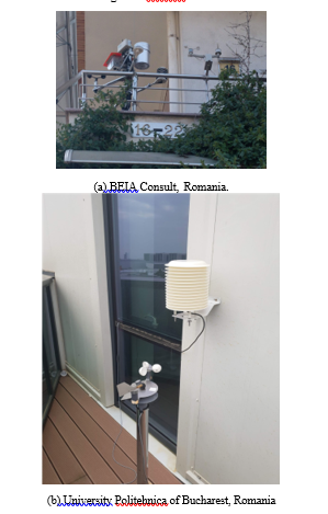Figure 2: Installed air-quality sensors that send the data the Tel-MonAer platform.

The platform registers every hardware device employed by the end-user, such as sensors or device gateways, with a unique ID. The data from the sensors is firstly received by the MQTT protocol, through a device gateway and then forwarded to a cloud gateway. The Tel-MonAer system is capable of simultaneously monitoring different air quality parameters such as SO₂, NOx, CO, O₃, PM₁₀, PM_2.5, as well as meteorological parameters (wind direction and speed, pressure, temperature, relative humidity).

The air quality data is currently being collected from IoT sensors in two locations: the premises of BEIA Consult International and University Politehnica Bucharest, as shown in Figure 2.

Tel-MonAer is designed to allow some specific features like availability and scalability. Moreover, the platform will permit further development. The architecture of the platform is based on microservices, because of the advantages of this model, such as independent, faster and more cost-effective development of each microservice and dedicated and specific databases for each component.

The high volumes of data stored by the Tel-MonAer platform demand a scalable and performant storage layer. For this purpose, Apache Cassandra database has been used because of its ability to scale almost linearly, to tackle failover situations and to automatically replicate data in more data centers.

The data is further processed by the platform, using two types of processing. Batch processing is used for analyzing the data received from multiple sensors and within a specific time frame and for performing predictions of possible evolutions. Real-time processing is used for event detection. We used Apache Spark, a general use engine for both real-time and batch processing, because of its advantages, such as in-memory processing, real-time stream processing and sophisticated analytics support.

3.2.  Details of the method used

The parameters of the data set used to perform the analysis are: PM10 and PM2.5 concentration values, atmospheric pressure, atmospheric temperature and relative humidity. The measurements were performed in Bucharest using Libelium sensors. The parameters were measured between the 1^st of November 2018 and the 28^th of January 2019, with a frequency of 15 minutes.

The process of data acquisition follows several steps: accessing the gateway interface, connecting to the MySQL database interface to access the sensor data, logging into the phpMyAdmin interface, querying the database for hourly average values, downloading the data selected by the query function.

4. Experimental Results

The dataset resulted from the registered measurements contains 2133 values for every parameter. Firstly, a qualitative analysis of the data has been performed, in order to compare the measured values with standard data requirements. Secondly, a preliminary analysis has been carried out using statistical descriptive methods for the parameter, such as variation, mean value and standard deviation [1].

The variation of PM₁₀ and PM_2.5 concentrations function of relative humidity is presented in Figure 3 and Figure 4, respectively. The results show an increase in PM concentrations for values of relative humidity greater than 90%. This is a strong indication of a measurement error, caused by the measurement method or by the complex chemistry of PMs.

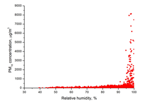Figure 3: PM₁₀ concentration vs relative humidity for the entire data set

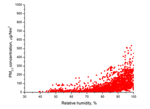Figure 4: PM_2.5 concentration vs relative humidity for the entire data set

Considering the need to ensure the accuracy of measurements and the previous measurement results, it is necessary to determine a threshold value of relative humidity from which the measurements accuracy decrease. For this purpose, Pearson’s correlation coefficients between relative humidity and PM concentrations were calculated for different data sub-sets. The results shown in Figure 5 indicate a stronger correlation for both types of PMs when relative humidity values are higher than 80%.

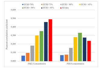Figure 5: The absolute values of Pearson’s correlation coefficients between PM_2.5 and humidity, respectively PM₁₀ and humidity, for selected data sub-sets.

In order to perform a comparative analysis, the absolute value of the correlation coefficients was used, and the threshold value of relative humidity was established at 80%. The dataset that resulted consists of 591 values and represents 27.7% of the total values registered.

The variation of measured PM₁₀ and PM_2.5 concentrations for the data sub-set corresponding to values of relative humidity lower than 80% are presented in Figure 6. For the same data sub-set, Figure 7 shows the PM₁₀ and PM_2.5 concentrations function of relative humidity.

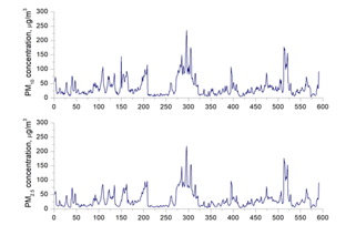Figure 6: Variation of measured values for PM₁₀ and PM_2.5 concentration for the data sub-set (humidity < 80%).

Figure 7: PM_2.5 and PM₁₀ concentration vs relative humidity for the data sub-set (humidity < 80%).

Table 1: Correction factors for humidity classes

Class name	Range of variation, (%)	Correction factor
K1	≤ 80	1
K2	80-85	1.5152
K3	85-90	2.3008
K4	90-95	3.3807
K5	95-98	6.6515
K6	> 98	14.4549

In order to make corrections that eliminate the influence of humidity on the values of PM concentrations, it is proposed a division by humidity classes for which the values of correction factors have been estimated. The correction factor values for humidity classes were calculated as average values of the corresponding correction factors for the humidity values of each variation interval. The resulting values are presented in Table 1.

4.1.  Algorithm for correcting concentrations of PM_2.5 and PM₁₀

Based on the information and data measured in the Tel-MonAer project, a correction algorithm (presented below) was developed for the concentration values of PM_2.5 and PM₁₀.

Step 1.	Determination of the correction factor for humidity Each measured value of the relative humidity falls into the corresponding humidity class (according to Table 1) and then the correction factor corresponding to the class is identified)
Step 2.	Correction for humidity of PMx concentration For each value of the PMx concentration measured, the following formula is applied: (1) Where: PMx – x fraction of particulate matter (e.g. PM2.5 and PM10); Conc PMx corr H – the value of PMx concentration as a function of humidity; Conc PMx measured – the value of the measured PMx concentration; FC – the value of the correlation factor.
Step 3.	Making the correction by reporting to the reference methods For each value of the concentration corrected in Step 2, the formula applies: (2) Where the function is specific to each type of sensor, pollutant and mediation period.
Step 4.	Calculation of the final concentration for the specified mediation interval. The average value of the corrected concentrations for the specified mediation periods (hour, day) is calculated.

For the application and testing of the calculation algorithm, the concentration data of PM_2.5, PM₁₀ and relative humidity acquired using a Libelium SCP station (with OPC-N3 sensor) was used. The station was installed outside the building of the CAMPUS Center, within the Politehnica University of Bucharest (Figure 8). The data set used corresponds to the period March 13-May 13, 2019.

The corrected values of the concentrations of PM_2.5 and PM₁₀ were calculated with the measurements made by the National Environmental Protection Agency, at the Morii Lake measuring point within the National Network for Air Quality Assessment (Figure 9).

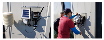Figure 8: Installation of the measuring equipment Libelium SCP at the CAMPUS center

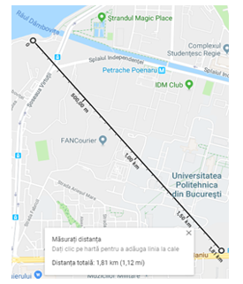Figure 9: Distance between the Morii Lake monitoring point and the CAMPUS monitoring point

The correction algorithm was applied for PM_2.5 and PM₁₀ and the results were compared with the values of the measured concentrations at Morii Lake measurement point in the National Air Quality Assessment network.

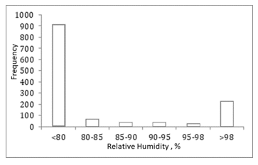Figure 10: Histogram of relative humidity for the test period

4.2.  Application of the algorithm for PM_2.5

During the analyzed period (March 13 – May 13, 2019), there were recorded hourly values of relative humidity (Figure 10) below 80% in 915 hours (69% of the total) and values greater than 98% in 231 hours (17.42%). Thus, the correction algorithm for humidity will lead to the modification of the values for 31% of the recorded values.

The hourly concentrations measured (Figure 11) during the testing phase of the algorithm recorded values below 7 μg / Nm³ in 32.43% of hours, values less than 22 μg / Nm³ being measured in 80.24% of the total number of hours. Also 43 values over 67 μg / Nm³ were recorded.

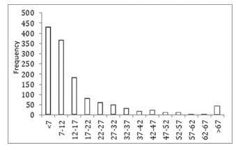Figure 11: Histogram of the values of PM_2.5 concentrations measured during the test period

By applying the algorithm, the very small values (below 7 μg / Nm³) of the measured concentrations were increased and represent 1.52% of the total. Values lower than 22 μg / Nm³ represent 83.45% of the total number of hours. The number of values greater than 67 μg / Nm³ was reduced to one value (Figure 12).

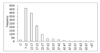Figure 12: Histogram of PM_2.5 concentration values corrected after applying the algorithm

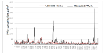Figure 13: Measured and corrected concentration values of PM_2.5 for the test period

Figure 13 shows the values of PM_2.5 concentrations measured and corrected for the test period. It is observed the elimination of the extreme values generated by the increase of humidity and the increase of the small values which represents the elimination of the underestimation of the measured values.

4.3.  Application of the algorithm for PM₁₀

The hourly concentrations measured (Figure 14) during the testing phase of the algorithm recorded values below 12 μg / Nm³ in 44.49% of the hours, values less than 44 μg / Nm³ being measured in 92.23% of the total number of hours. Also, 33 values of over 92 μg / Nm³ were recorded.

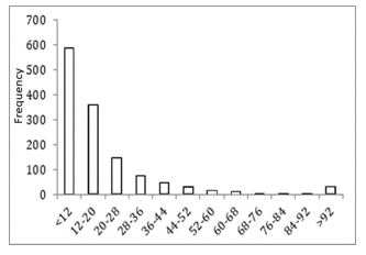Figure 14: Histogram of PM₁₀ concentration values measured during the test period

By applying the algorithm, the very small values (below 12 μg / Nm³) of the measured concentrations were increased and represent 0.5% of the total. The number of concentrations greater than 92 μg / Nm³ was reduced to a single value (Figure 15).

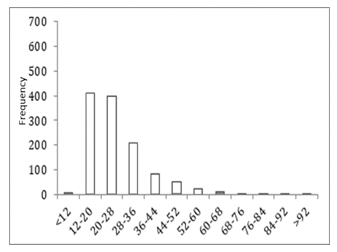Figure 15: Histogram of PM₁₀ concentration values corrected after applying the algorithm

The following figure shows the values of PM₁₀ concentrations measured and corrected for the test period. It is observed the elimination of the extreme values generated by the increase of humidity and the increase of small values which represents the elimination of the underestimation of the measured values (Figure 16).

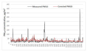Figure 16: Values of concentrations measured and corrected by PM₁₀ for the test period

4.4.  Performance evaluation of the algorithm

The monitoring station at Morii Lake is urban-background type, the measured values being representative on an area with a radius of 1-5 km around the station. The CAMPUS Center where the Libelium sensors were located is within the representative area (1.8 km from the station). By placing it at a higher height, the effect of the pollution generated by car traffic was reduced, but it is also possible to reduce the measured values due to the height at which they were located.

The hourly PM_2.5 concentrations measured at the monitoring station at Morii Lake (Figure 17) were below the value of 22 μg / Nm³ in 82.69% of the total number of hours.

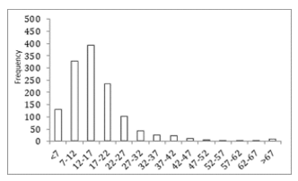Figure 17: Histogram of the values of PM_2.5 concentrations measured at the Morii Lake point from the National Air Quality Network

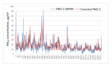Figure 18: Values of corrected PM_2.5 concentrations and those measured by ANPM for the test period

The comparative graphical representation of the values of the corrected PM_2.5 concentrations and those measured by ANPM (Figure 18) during the testing period of the algorithm indicates close values and similar evolution trend.

The hourly PM₁₀ concentrations measured at the Morii Lake monitoring station (Figure 19) were below the value of 44 μg / Nm³ in 94.94% of the total number of hours.

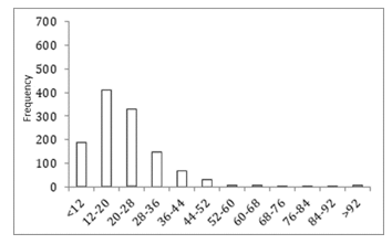Figure 19: Histogram of the values of PM₁₀ concentrations measured at the Morii Lake point from the National Air Quality network

The comparative graphical representation of the values of the corrected PM₁₀ concentrations and those measured by ANPM (Figure 20) during the testing period of the algorithms indicates close values and similar evolution trend.

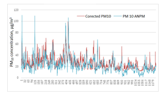Figure 20: Values of corrected and officially measured concentrations of PM₁₀ for the test period

The efficiency of the correction algorithm was evaluated at this stage by the value of the Pearson correlation coefficients (Table 2).

Table 2: Pearson’s correlation coefficient values for the analyzed data sets

Concentration	Correlation coefficient
	Measured values vs. ANPM values	Corrected values vs. ANPM values
PM2.5	0.268	0.688
PM10	0.216	0.663

This shows a 2.5-fold increase in the correlation coefficient for PM_2.5 concentrations, from a value of 0.268 (Libelium measured data vs. ANPM measured data).

For PM₁₀ concentrations, the value of the correlation coefficient increased 3-fold, from 0.216 (Libelium measured data vs ANPM measured data) to 0.663 (Libelium corrected data vs. ANPM measured data).

5. Conclusions and Future Work

The influence of relative humidity on the PMs concentration values is significant for the devices based on laser measurement technology. For this type of IoT devices we propose a threshold value for relative humidity of 80% under which to consider PMs measured concentration as valid. For the situation when relative humidity has values over 80%, a specific algorithm was developed. The algorithm corrects the PMs measured values considering the type of the sensors and the value of humidity.

The correction algorithm was tested on a data set containing PMs concentration values and other meteorological parameters for a period of two months. The results show an increase of at least 2.5 times of the correlation coefficient between the corrected values and those measured by the reference station of the National Air Quality Monitoring Network.

Future work will consider further testing of the algorithm and the development of a specific ML algorithm for air quality predictions.

Conflict of Interest

The authors declare no conflict of interest.

Acknowledgment

The work presented in this paper has been funded by Tel-MonAer project subsidiary contract no.1223/22.01.2019, from the NETIO project ID: P_40270, MySmis Code: 105976 and by the WINS@HI project, PN-III-P3-3.5-EUK-2017-02-0038.

1.  CSCS19: The 22nd International Conference on Control Systems and Computer Science, 28-30 May 2019, Faculty of Automatic Control and Computers, University Politehnica of Bucharest, Romania. https://cscs22.hpc.pub.ro/
2. J. Ayres, “The mortality effects of long-term exposure to particulate air pollution in the United Kingdom,” Report by the Committee on the Medical Effects of Air Pollutants, 2010.
3. P. J. Landrigan, R. Fuller, N. J. Acosta, O. Adeyi, R. Arnold, A. B. Bald´e, R. Bertollini, S. Bose-O’Reilly, J. I. Boufford, P. N. Breysse et al., “The lancet commission on pollution and health,” The Lancet, vol. 391, no. 10119, pp. 462–512, 2018.
4.  V. Hadjioannou, C. X. Mavromoustakis, G. Mastorakis, J. M. Batalla, I. Kopanakis, E. Perakakis, and S. Panagiotakis, “Security in smart grids and smart spaces for smooth IoT deployment in 5g,” in Internet of Things (IoT) in 5G Mobile Technologies. Springer International Publishing, 2016, pp. 371–397. [Online]. Available: https://doi.org/10.1007%2F978-3-319-30913-2 16
5.  M. Ianculescu, A. Alexandru, and E. Tudora, “Opportunities brought by big data in providing silver digital patients with ICT-based services that support independent living and lifelong learning,” in 2017 Ninth International Conference on Ubiquitous and Future Networks (ICUFN). IEEE, jul 2017. [Online]. Available: https://doi.org/10.1109%2Ficufn.2017.7993817
6. J. M. Batalla, K. Sienkiewicz, W. Latoszek, P. Krawiec, C. X. Mavromoustakis, and G. Mastorakis, “Validation of virtualization platforms for i-IoT purposes,” The Journal of Supercomputing, vol. 74, no. 9, pp. 4227–4241, aug 2016. [Online]. Available: https://doi.org/10.1007%2Fs11227-016-1844-2
7.  J. S. Apte, K. P. Messier, S. Gani, M. Brauer, T. W. Kirchstetter, M. M. Lunden, J. D. Marshall, C. J. Portier, R. C. Vermeulen, and S. P. Hamburg, “High-resolution air pollution mapping with google street view cars: exploiting big data,” Environmental science & technology, vol. 51, no. 12, pp. 6999–7008, 2017.
8. D. Fecht, A. L. Hansell, D. Morley, D. Dajnak, D. Vienneau, S. Beevers, M. B. Toledano, F. J. Kelly, H. R. Anderson, and J. Gulliver, “Spatial and temporal associations of road traffic noise and air pollution in london: Implications for epidemiological studies,” Environment international, vol. 88, pp. 235–242, 2016.
9. H.Lin,T.Liu,J.Xiao,W.Zeng,L.Guo,X.Li,Y.Xu,Y.Zhang,J.J. Chang, M. G. Vaughn et al., “Hourly peak pm 2.5 concentration associated with increased cardiovascular mortality in guangzhou, china,” Journal of Exposure Science and Environmental Epidemiology, vol. 27, no. 3, p. 333, 2017.
10. T. Watkins, “Draft roadmap for next generation air monitoring,” Environmental Protection Agency, 2013.
11.  K.-H. Kim, E. Kabir, and S. Kabir, “A review on the human health impact of airborne particulate matter,” Environment international, vol. 74, pp. 136–143, 2015.
12. A. Y. Watson, R. R. Bates, D. Kennedy et al., Air pollution, the automobile, and public health. National Academies, 1988.
13.  S. Holgate, J. Grigg, R. Agius, J. R. Ashton, P. Cullinan, K. Exley, D. Fishwick, G. Fuller, N. Gokani, C. Griffiths et al., “Every breath we take: The lifelong impact of air pollution, report of a working party.” Royal College of Physicians, 2016.
14.  F. Dominici, R. D. Peng, M. L. Bell, L. Pham, A. McDermott, S. L. Zeger, and J. M. Samet, “Fine particulate air pollution and hospital admission for cardiovascular and respiratory diseases,” Jama, vol. 295, no. 10, pp. 1127–1134, 2006.
15.  J. G. Watson, J. C. Chow, H. Moosm¨uller, M. Green, and N. Frank, “Guidance for using continuous monitors in pm2. 5 monitoring networks,” Nevada Univ. System, Desert Research Inst., Reno, NV (United States , Tech. Rep., 1998.
16.  B. Zhang, L. Jiao, G. Xu, S. Zhao, X. Tang, Y. Zhou, and C. Gong, “Influences of wind and precipitation on different-sized particulate matter concentrations (pm 2.5, pm 10, pm 2.5–10),” Meteorology and Atmospheric Physics, vol. 130, no. 3, pp. 383–392, 2018.
17.  K. Y. Ng and N. Awang, “Quantile regression for analysing pm10 concentrations in petaling jaya,” Malaysian Journal of Fundamental and Applied Sciences, vol. 13, no. 2, 2017.
18.  C. Lou, H. Liu, Y. Li, Y. Peng, J. Wang, and L. Dai, “Relationships of relative humidity with pm 2.5 and pm 10 in the yangtze river delta, china,” Environmental monitoring and assessment, vol. 189, no. 11, p. 582, 2017.

(Click Here)

(Click Here)