1. Introduction

This paper is an extension of work based on Machine Learning Techniques for Big Data Analytics originally presented in 2019 9th International Conference on Cloud Computing, Data Science & Engineering (Confluence) [1]. Weather prediction is one of the vital applications of technology to forecast the atmosphere for the future and has its wide application in number of domains such as forecasting air flights delay, satellites launching, crop production, natural calamities etc. Weather prediction can be classified into 4 categories depending on the time of forecast : a) Very Short Term Prediction: forecast for few hours in advance b) Short Term: forecast for days in advance c) Medium Term: forecast for weeks in advance d) Long Term: for months-years in advance. In the early days, data collected from several weather stations were fed into some numerical models which made the use of statistics to predict the future. While with the growing popularity and tremendous applications of Machine Learning Techniques, availability of high speed processors, new improved tools and techniques, researchers are now experimenting with ML techniques in meteorological domain too.

Neural Networks is one of the most popular Machine Learning techniques but it lacked its popularity in the late 90’s due to gradient descent problem and limited processing power of the computers leading to very high learning time. As the technology progressed further, various techniques like parallel processing, High Performance Computing clusters, GPUs etc. have been developed which when applied in NN results in tremendous improvement of their performance.

RNN are the recurrent neural networks with the feedback connection but they might get trapped in Vanishing Gradient Problem. LSTM (Long Short Term Memory neural networks, introduced by Hochreiter and Schmidhuber in 1997) are gated RNNs which overcomes the above-mentioned issue by creating the gradients that neither explode nor vanish with time. It is composed of 1 memory unit and 3 gates namely input, output and forget gate which uses sigmoid activation function to decide which information they need to input, output and forget. LSTM has self-loops with conditioned weights controlled by forget gate to generate paths where gradient can flow for greater time [2]. It has also an advantage of learning long term dependencies, thereby widely used in text sequencing domain. Architecture of LSTM networks has been described in Figure 1. LSTMs are trained using BPTT i.e. Back Propagation through Time, thus overcomes vanishing gradient problem but it might get stuck in local optima.

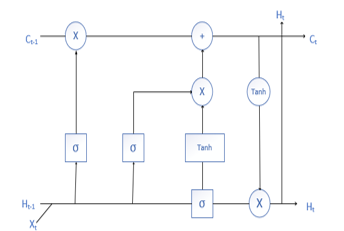Figure 1: Architecture of LSTM: Image Source [3]

2. Literature Review

In this section, a detailed review has been conducted on work done by various researchers for application of NN in the field of weather prediction. A study on various Data Mining algorithms popularly used in the field of weather prediction has been conducted and several challenges that may occur while applying traditional data mining techniques were highlighted [4]. In [5], the authors analyzed 30 years of Hong Kong metrological data using 5 layered Deep NN with 4 layered Stacked Auto Encoders to learn raw data features with SVR for prediction. NMSE (Normalized Mean Square Error), R Square and DS (Directional Symmetry) metrics have been used for evaluation purpose. In [6], the reviewers analyzed weather data collected from www.weatherunderground.com which was first normalized and then fed to 3 layered BPNN model to obtain non-linear relationships.

IGRA dataset collected across 60 stations was analyzed by authors to design data driven kernel and to provide an efficient inference procedure [7]. Best validation results were obtained using 2 stacked RBM with hidden neurons 50 and 150. In [8], the authors used CNN for the first time to predict monthly rainfall of Australia and the results proved that CNN performs better in comparison to prediction model used by Bureau of Meteorology and MLP for months with high annual average rainfall. Researchers also proposed CFPS-HGA (Climate features and neural network parameters selection-based hybrid genetic algorithm) for setting neural network parameters and the proposed algorithm performed better [9].

Meteorological data collected from BKMG (for the period 1973-2009) and ENSO data from NOAA was analyzed by researchers using RNN, CRBM and Convolutional Networks [10]. In [11], the authors implemented NARX NN (Non Linear Auto regressive with exogenous variables), a type of recurrent NN for predicting multiple weather attributes and the results concluded that proposed algorithm performed better than CBR (Case Based Reasoning). In [12], researchers proposed a new layer i.e. Dynamic Convolutional layer which used filter in addition to feature maps from the previous layer to predict the sequence of rain radar images using Caffe library and Stochastic Gradient Decent optimizer.

In [13], the researchers compared the performance of deep neural NN with shallow NN for short term wind prediction. NN parameters were reduced using PMI (Partial Mutual Information) based IVS algorithm and the results proved that 3 layered stacked auto encoders performed better. In [14], the authors proposed Deep Multilayer Perceptron using Cascade learning and implanted it on H1-B Visa applications record and cardiac dataset and the results proved that proposed model has less run time and greater accuracy.

In [15], the authors proposed 2 layers stacked LSTM model (each layer has independent LSTM model for every location) for weather data obtained from Weather Underground website from 2007 to 2014. In [16], the authors compared the performance of ARIMA model and LSTM (weather variables are combined) on weather data collected from Weather Underground for the period 2012 to 2016 and it was concluded that LSTM performs better than ARIMA.

In [17], the authors proposed deep LSTM model for wind prediction on the data from Manchester Wind Farm for 2010-2011 and the proposed algorithm performed better than BPNN and SVM. Best results were obtained from the model consisting of 3 hidden layers constituting 300, 500 and 200 neurons. In [18],   15 years of hourly meteorological data for 9 cities in Morocco was analyzed by authors using multi-stacked LSTM to forecast 24 and 72 hours weather data. Missing values were eliminated using forward filling and RMSProp optimizer was used.

3. Experimental Study

As per the survey done in Section 2, it can be concluded that LSTM is one of the most popular and successfully used technique in the domain of weather prediction. Thus, in this experimental study, multi-stacked LSTM model has been implemented on Spark platform to determine the best architecture for the task of weather prediction. For the analysis purpose, dataset of 2 GB from INMET (National Meteorological Institute – Brazil) has been used which consists of hourly weather data from 122 weather stations of various south-eastern states of Brazil i.e. Rio de Janeiro, Sao Paulo, Minas Gerais and Espirito Santo from 2000 to 2016 [19]. Brazil is the largest country in the South America and its temperature rarely fall below 20 degrees. In the proposed experiment, a computer with 1TB memory, 16 GB RAM and 1.8 GHz processor has been used. Dataset includes 31 features and around 9.7 million (9,779,168) rows. All the dataset is first loaded into the Spark dataframe and unnecessary columns i.e. wsnm, wsid, elvt, lat, lon, inme, city, prov, mdct, date, yr, mo, da, hr, tmax, tmin have been deleted from our schema (Only 15 attributes have been preserved as mentioned in Table 1).

Data pre-processing is the pre-requisite of any analytics process. All the null values have been replaced with zero and the results are cited in Table 2. Several other ways to deal with null values are as follows: a) Replace nulls with zero in case of numerical attributes b) Replace with mean/median/mode values c) Use algorithms that support missing values d) Remove the rows having null values.

Table 1: Attributes for weather prediction

Attribute	Description
Prcp	Amount of precipitation in millimeters (last hour)
Stp	Air pressure for the hour in hPa to tenths (instant)
Smax	Maximum air pressure for the last hour in hPa to tenths
Smin	Minimum air pressure for the last hour in hPa to tenths
Gbrd	Solar radiation KJ/m2
Temp	Instant Air Temperature (Celsius degrees)
Dewp	Instant Dew Point (Celsius degrees)
Dmax	Maximum Dew Point (Celsius degrees)
Dmin	Minimum Dew Point Temperature (Celsius degrees)
Hmdy	Relative Humidity of Air (%
Hmax	Maximum Relative Air Humidity (%)
Hmin	Minimum Relative Air Humidity (%)
Wdsp	Instant Wind Speed (meters per second)
Wdct	Wind direction in radius degrees (0-360)
Gust	Wind Gust Intensity (meters per second)

Input to the proposed LSTM network is prcp, stp, smax, smin, gbrd, dewp, dmax, dmin, hmdy, hmax, hmin, wdsp, wdct, gust, temp at (t-1)^th hour and the output is temperature at (t)^th  hour and at (t+24)^th hour. Architecture of the proposed network has been described in Figure 2. Input attributes are normalized between 0 and 1 via pyspark.ml.MinMaxScaler and training and validation data has been split in the ratio 80:20.

4. Experimental Results

Let I, H and O be the number of neurons in input layer, hidden layer and output layer respectively. Models are trained using Keras module (with Tensorflow backend) which has dense library for implementing LSTM networks. Weights to be optimized in the LSTM networks are as follows:

W1=4*I*H;                  U1=4*H*H;

B1=4*H;       W2=H*O;

B2=O      …..(1)

For H=5 (5 units in LSTM with 1 hidden layer), I=15 (15 input attribute) and O=1 (1 output attribute), W1= 4*5*15=300, U1=4*5*5=100, B1=4*5=20, W2= 5*1=5, B2=1. Thus, there are total of 426 parameters which needs to be optimized.

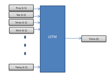Figure 2: Architecture of LSTM network

Table 2: Number of nulls

Attributes	Number of null values
Prcp	8371184
Stp	0
Smax	0
Smin	0
Gbrd	4108820
Dewp	475
Dmax	310
Dmin	807
hmdy	0
Hmax	12
Hmin	44
Wdsp	925561
Wdct	0
Gust	316474
Temp	31

Two separate networks have been implemented, one provides output temperature at t^th hour and the other network provides output at (t+24)^th hour. In the proposed study, the number of hidden neurons has been varied from 10 to 30 and the number of   hidden layers has been increased up to 3. Results of both the case studies have been mentioned in Table 3. Performance of Adam (Adaptive Moment Estimation), SGD (Stochastic Gradient Decent) and RMSProp (Root Mean Square Prop) optimizers has also been compared for 2 hidden layers comprising 10 and 20 neurons respectively for 24 hours’ time lag and results are described in Table 4. From the results, it can be concluded that Adam optimizer performs best whereas SGD performs worst. Thus, Adam optimizer has been used in all the implemented case studies. Mean Absolute Error (MAE) metrics has been used for the evaluation purpose. Run time of the network (in floating point number) has also been analyzed to determine the complexity of the network.

Table 3: MAE of LSTM networks with 1 hour and 24-hour time lag

S. No	Number of hidden layers	Number of hidden units	Iterations	1 hour time lag		24 hour time lag
				MAE	Runtime	MAE	Runtime
1	1	10	100	0.015151	28041.47	0.041649	30256.38
2	1	20	100	0.015462	29292.39	0.041582	29889.34
3	1	30	100	0.015365	30854.15	0.042124	28289.06
4	2	10,10	100	0.015088	48892.43	0.040463	49878.65
5	2	20,20	100	0.015077	49898.42	0.040839	46737.57
6	2	30,30	100	0.015259	50805.43	0.040060	46829.74
7	2	10,20	100	0.015124	42302.25	0.040020	52487.23
8	3	10,10,10	100	0.015269	124915.8	0.040546	101543.68

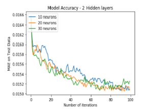Figure 3: MAE of LSTM with 2 hidden layers for 1-hour time lag

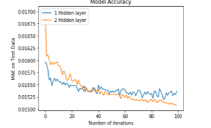Figure 4: MAE with 1 and 2 hidden layers, each having 30 neurons each for 1 hour time lag

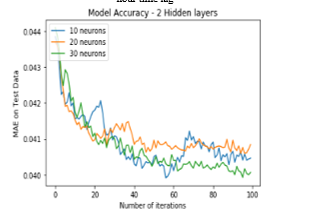Figure 5: MAE of LSTM with 2 hidden layers for 24-hour time lag

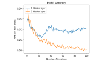Figure 6: MAE with 1 and 2 hidden layer, each having 30 neurons each for 24 hour time lag

Table 4: comparison of MAE for various optimizers for 24-hour time lag

Optimizers/Metric	MAE	Accuracy	Runtime
Adam	0.04002	6.64686E-06	52487.2306
Rmsprop	0.05972	5.62427E-06	51896.5460
SGD	0.04142	6.64686E-06	40895.8979

From the experimental results as mentioned in Table 3, it can be inferred that increasing the number of hidden layers in the network increases the accuracy (network with low MAE value has greater accuracy) of the network i.e. increasing the number of hidden layers from 1 to 2 improves the accuracy of the network. At the same time, time complexity of the network is also increased by marginal amount (can be interpreted from runtime as mentioned in Table 3).

Figure 3 and Figure 5 illustrates the comparison of MAE with 2 hidden layers comprising 10, 20 and 30 neurons each for 1 hour time lag and 24 hour time lag respectively over 100 iterations. For 1 hour time lag, network with 2 hidden layers comprising 20 neurons each provides best results (with the  lowest MAE value of  0.015077 as stated in Figure 3) whereas for 24 hour time lag, network with 2 hidden layers comprising 10 and 20 neurons respectively provides best results with the MAE value of 0.040020.

Figure 4 shows the comparison for networks of 1 hidden layer having 30 neurons with the network of 2 hidden layers comprising 30 neurons each for 1 hour time lag and it can be inferred that network with 2 hidden layers has low MAE value as compared to network with 1 hidden layer. Similarly, Figure 6 shows comparison for networks of 1 hidden layer having 30 neurons with the network of 2 hidden layers comprising 30 neurons each for 24 hour time lag and it can be inferred that network with 2 hidden layers has low MAE i.e. 0.040060 value as compared to network with 1 hidden layer i.e. MAE value of 0.042124.

From the case studies implemented, it can also be observed that MAE for 1 hour time lag is comparatively low, thus gives more accurate results as compared to network with 24 hour time lag i.e. network with short term predictions provides higher accuracy as compared to network with medium term predictions.. More combinations of the hidden neurons and layers can be explored in the near future to obtain better results.

5. Conclusion and Future Work

In this paper, Deep LSTM network has been implemented on 15 years meteorological data. Number of hidden layers has been increased up to 3 and it can be concluded that increasing the number of hidden neurons in the layer does not necessarily increases the accuracy of the model as network might start learning the linear relationship between the attributes. Also, increase in the number of layers in the model increases the run time of network by marginal amount, thus increasing the complexity of the network.

There are number of combinations possible for choosing the adequate number of hidden neurons and hidden layers in the network which can provide the minimum MAE. Manually testing all such combinations will be a quite tedious task. Thus, process of selection of number of hidden layers and hidden neurons needs to be automated.

Also, the algorithm takes quite longer time to run on single CPU. Thus, it becomes hard to increase the number of hidden layers and neurons beyond a significant point. Parallel processing of neural network might help us in reducing the time complexity of the network. Time complexity can further be reduced by employing more number of processors to do a task or by using the high speed GPUs. In future, it would be interesting to study the reduction in time complexity by implementing the above algorithms on increased number of processors and on GPUs.

Conflict of Interest

The authors declare no conflict of interest.

1.  S. Mittal, O.P. Sangwan,“Big Data Analytics using Machine Learning Techniques” in 2019 9th International Conference on Cloud Computing, Data Science & Engineering (Confluence), Noida, India. http://dx.doi.org/ 10.1109/CONFLUENCE.2019.8776614.
2.  I. Goodfellow, Y. Bengio, A. Courville, Deep Learning, MIT Press, 2016.
3.  https://en.wikipedia.org/wiki/Long_short-term_memory.
4.  S. Mittal, O.P. Sangwan,“ Big Data Analytics Using Data Mining Techniques: A Survey” in book: Advanced Informatics for Computing Research,264-273, 2018 Second International Conference, ICAICR, Shimla, India. http://dx.doi.org/ 10.1007/978-981-13-3140-4_24.
5.  J. Liu, Y. Hu, J. Jia You, P. Wai Chan,“Deep Neural Network Based Feature Representation for Weather Forecasting” in 2014 International Conference on Artificial Intelligence (ICAI), Las Vegas, Nevada, USA.
6.  Ch. J. Devi, B.S. Prasad Reddy, K.Vagdhan Kumar, B.Musala Reddy, N. Raja Nayak,“ANN Approach for Weather Prediction using Back Propagation” International Journal of Engineering Trends and Technology, 3(1), 20-23, 2012.
7.  A. Grover, A. Kapoor, E. Horvitz,“A Deep Hybrid Model for Weather Forecasting” in 2015 21th ACM SIGKDD International Conference on Knowledge Discovery and Data Mining, KDD, 379-386, Sydney, NSW, Australia. http://dx.doi.org/10.1145/2783258.2783275.
8. A. Hiader, B. Verma,“Monthly Rainfall Forecasting using One-Dimensional Deep Convolutional Neural Network,” IEEE Access, 6, 69053 – 69063, 2018. http://dx.doi.org/10.1109/ACCESS.2018.2880044.
9. A. Hiader, B. Verma,“A novel approach for optimizing climate features and network parameters in rainfall forecasting” Soft Computing, Springer, 22(24), 2018. https://doi.org/10.1007/s00500-017-2756-7.
10.  A. Galih Salman, B. Kanigoro, Y. Heryadi,“Weather forecasting using deep learning techniques” in 2015 International Conference on Advanced Computer Science and Information Systems (ICACSIS), Depok, Indonesia. http://dx.doi.org/10.1109/ICACSIS.2015.7415154.
11.  S. Biswas, N. Sinha, B. Purkayastha, L. Marbaniang,“Weather prediction by recurrent neural network dynamics” Int. J. Intelligent Engineering Informatics, 2(2/3), 166-180, 2014. http://dx.doi.org/10.1504/IJIEI.2014.066208.
12.  B. Klein, L. Wolf, Y. Afek,“A Dynamic Convolutional Layer for Short Range Weather Prediction” in 2015 IEEE, Conference on Computer Vision and Pattern Recognition (CVPR). Boston, MA, USA. http://dx.doi.org/ 10.1109/CVPR.2015.7299117
13.  M. Dalto, J. Matusko, M. Vasak,“Deep neural networks for ultra-short-term wind Forecasting” in 2015 IEEE, International Conference on Industrial Technology (ICIT), Seville, Spain. http://dx.doi.org/ 10.1109/ICIT.2015.7125335.
14.  A. Gupta ,H. Kumar Thakur , R. Shrivastava, P. Kumar, S. Nag, “Big Data Analysis Framework Using Apache Spark and Deep Learning” in 2017 IEEE, International Conference on Data Mining Workshops (ICDMW), New Orleans, LA, USA. http://dx.doi.org/ 10.1109/ICDMW.2017.9.
15. Z. Karevan, J. Suykens,“Spatio-temporal Stacked LSTM for Temperature Prediction in Weather Forecasting” Cornell University, 2018.
16. A. Galih Salman, Y. Heryadi, E. Abdurahman, W. Suparta,“Weather Forecasting Using Merged Long Short-Term Memory Model (LSTM) and Autoregressive Integrated Moving Average (ARIMA) Model” Journal of Computer Science, 14(7), 930-938, 2018. https://doi.org/10.3844/jcssp.2018.930.938
17.  Q. Xiaoyun, K. Xiaoning, Z. Chao, J. Shuai, M. Xiuda,“Short-Term Prediction of Wind Power Based on Deep Long Short-Term Memory” in 2016 IEEE, PES Asia-Pacific Power and Energy Engineering Conference (APPEEC), Xi’an, China.http://dx.doi.org/10.1109/APPEEC.2016.7779672.
18. M. Akram Zaytar, C. El Amrani,“Sequence to Sequence Weather Forecasting with Long Short-Term Memory Recurrent Neural Networks” International Journal of Computer Applications, 143(11), 2016. http://dx.doi.org/10.5120/ijca2016910497.
19. https://www.kaggle.com/PROPPG-PPG/hourly-weather-surface-brazil-southeast-region.

(Click Here)

(Click Here)