1. Introduction

This paper is an extension of work originally presented in the conference Proceedings of the IEEE 17st World Symposium on Applied Machine Intelligence and Informatics, (SAMI 2019) [1].

1.1        Wireless Sensor Networks

Wireless sensor networks (WSNs), a technology operating in an unattended ad-hoc mode, may be formed by hundreds to thousands autonomous sensor nodes¹, example shown in Figure 1, to gather information from the adjacent environment and to detect certain events of interest over the monitored area (e.g., buildings, homes, forests, oceans, mountains, etc.) [2–5]. Over the past years, this technology has found the application in many different areas, e.g., disaster detection, industrial monitoring, health assistance, military surveillance, etc. [6]. Therefore, the design of the sensor nodes has to be adapted to environmental conditions (e.g., the sensor nodes for underground operation have an increased transmission power whereby noisy channel attenuations can be overcome) [3]. However, as these sensor nodes are simple and low-cost devices, they suffer from limited energy capacity and computation capabilities, resulting in decreased robustness to potential threads such as radiations, pressure, temperature, attacks, etc. [7–9]. Thus, many of the real-life WSN-based applications are equipped with data aggregation mechanisms for suppressing or even overcoming the impacts of these negative factors on the operation of WSNs. Moreover, data aggregation can eliminate highly correlated and duplicated information as well [8].

1.2        Data Aggregation

In general, data aggregation poses any process in which data from multiple sources is transformed into a summary form for further statistical processing or analyzing. The data aggregation mechanisms are designed to process measured information from multiple independent sensor nodes in order to provide a greater quality of servise (QoS) [8]. Xiao et al. define two categories of the data aggregation mechanisms, namely [9]:

Figure 1: Example of WSNs – Memsic’s classroom kit (Source: Reprinted from [13])

In the centralized data aggregation schemes, the sensor nodes transmit their measured information to a fusion center either directly or by multi-hop communication. In the second scenario, each sensor node has to establish and update the table with routing information, which is not a too effective way to deliver information to a fusion center over mobile networks and networks with limited energy sources such as WSNs [9]. Therefore, the distributed schemes are more frequently applied nowadays [10–13]. In these schemes, the adjacent sensor nodes communicate with each other and update their states according to the collected data [14]. Thus, a fusion center is not necessary for data aggregation as well as the sensor nodes know only local information whereby data aggregation is significantly simplified. In [15], Jesus et al. divide distributed aggregation schemes into three groups in terms of the communication perspective:

• Structured
• Unstructured
• Hybrid

Structured algorithms are dependent on network topologies and routing algorithms and therefore are not appropriate for mobile systems. Moreover, a single point of failure (e.g., a dead node, a link failure) can have a fatal impact on a whole system, especially in sparsely connected topologies such as tree-based structures. The next category, Unstructured algorithms, is independent of network topology and structure unlike the first category, and thus, network topology does not have to be predefined. These algorithms are characterized by simplicity, high scalability, high robustness, etc. The last category, i.e., Hybrid algorithms, utilizes strengths and suppress weaknesses of the previous approaches by their combination.

In terms of the computation perspective, the distributed data aggregation mechanisms can be classified as follows [15]:

• Computation of decomposable functions
• Computation of complex functions
• Counting

As mentioned earlier, we focus our attention on linear consensusbased algorithms for distributed summing, which can be classified as unstructured algorithms for computation of decomposable functions. These algorithms have significantly attracted the attention of the academy recently [16–18]. In [19], Gutierrez-Gutierrez et al. define two categories of these algorithms, namely:

• Deterministic
• Stochastic

From this set of the algorithms, we choose deterministic linear average consensus (referred to as AC), characterized by a variable mixing parameter , for distributed summing [20].

A properly configured stopping criterion can significantly optimize data aggregation over WSNs; therefore, its implementation is an essential complement for distributed data aggregation mechanisms. As mentioned above, we assume that the execution of the examined algorithm is bounded by a stopping criterion in our analyzes.

1.3        Summary of Contribution

In this paper, we analyze AC for distributed summing whose execution is bounded by a stopping criterion. We vary its initial configuration and the configuration of the analyzed stopping criteria (we examine a centralized and a fully-distributed one) in order to identify which configurations ensure the highest performance of the examined algorithm and in order to compare the analyzed stopping criteria in terms of the precision and the convergence rate. As mentioned earlier, a properly configured stopping criterion and algorithm optimize data aggregation, thereby saving energy, reducing the computation/the communication requirements, prolonging the network lifetime, etc.

In this paragraph we clarify the novelty of the presented paper in a comparison with the existing work presented in [1]: In [1], we analyze AC bounded by the fully-distributed stopping criterion defined in [13] – we vary the mixing parameter and the parameters of the implemented stopping criterion in order to identify the best-performing initial configurations of both the algorithm and the stopping criterion. In that paper, the inner states are multiplied by the network size before AC begins. In this paper, we compare these results with the scenario when the inner states are multiplied after AC is completed. The goal of this contribution is to identify when it is the most optimal to carry this multiplication out in terms of the precision and the convergence rate expressed as the iteration number for the consensus achievement. Furthermore, we also analyze the performance of the centralized stopping criterion from [6] and compare it with the results from [1] and the results from the extended analysis presented in this paper in order to identify which stopping criterion achieves higher performance.

1.4        Paper Organizanization

The paper is organized as follows: Section 2 is concerned with theoretical insight into the topic, i.e., we provide a mathematical model of AC and WSNs, the convergence conditions, and an explanation of the analyzed stopping criteria. Section 3 deals with the applied methodology and the used metrics for performance evaluation. Section 4 consists of the experimentally obtained results and a consecutive discussion. Conclusions are presented in Section 5.

2. Theoretical Background

The primary purpose of AC is to estimate the arithmetic mean from all the initial states. However, it can fulfill also other functionalities – in this paper, we analyze AC for distributed summing, i.e., the sum from all the initial states is estimated. In this case, the information about the network size n is necessary to be known by each sensor node, and the inner states have to be multiplied by this value, otherwise, the arithmetic mean is estimated instead of the sum [1].

2.1        Model of AC for Distributed Summing in WSNs

We model WSNs as simple finite graphs determined by the vertex and the edge sets, i.e., G = (V, E) [20]. The vertex set V is formed by all the graph vertices, which represent the sensor nodes in a network, i.e., V = {v₁, v₂, … v_n}. The graph order is equal to the number of the sensor nodes in a network, and so, |V| = n. Two vertices v_i and v_j are adjacent when they are connected to one another by an edge, i.e., e_ij ∈ E.

In AC, each vertex v_i stores and update its inner state x_i(k)^[1], represented by a scalar value – the inner states are initiated by for example a local measurement. After the initialization, the inner states asymptotically converge to the arithmetic mean from all the initial inner states by being updated at each iteration, as described in 1, [21]:

Here, x(k) is a variant column vector gathering all the inner states at the corresponding iteration, and W poses the weight matrix, affecting many aspects of the algorithm such as the convergence rate of the algorithm, the initial configuration, meeting/violating the convergence conditions, etc. [22]. As already stated, the inner states asymptotically converge to the estimated aggregate function, which can be expressed using 2, [21]:

Here, 1 represents a column all-ones vector formed by n elements. The algorithm works correctly iff the limit from (2) exists, which is ensured by meeting these convergence conditions described by 3–5, [21], [23,24]:

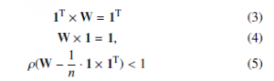
One of the ways to configure the weight matrix W is to allocate a constant value^[2] to all the edges in a graph. Such a matrix is referred to as the Peron Matrix and is defined by 7, [25]:

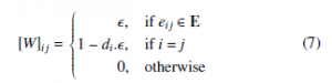
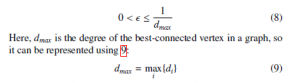
Here, d_i is the degree of the corresponding vertex, i.e., the number of its neighbors. As discussed in [23], the convergence of the algorithm is ensured in each non-bipartite non-regular graph when the mixing parameter  is selected from the interval described in 8:

2.2        Analyzed Stopping Criteria

In this subsection, we introduce the implemented stopping criteria for bounding the execution of AC.

The first analyzed stopping criterion is proposed in [13] and poses a fully-distributed approach, i.e., no global information is necessary for its proper functioning. It is determined by two constants, namely accuracy and counter threshold, which are the same for each sensor node and preset before AC begins. Moreover, each sensor node has its own counter, which is initiated with ”0” at each node. The principle of the stopping criterion is based on the calculation of the finite difference between the inner states at two consecutive iterations. If the finite difference is smaller than accuracy, the corresponding sensor node increments its counter by ”1”. If not, counter is reset^[3] regardless of its current value. When the finite difference is smaller than accuracy more times^[4] in a row, the algorithm is completed at the corresponding sensor node. Thus, this sensor node does not participate in AC and update its inner state any longer.

The other implemented stopping criterion from [6] is a centralized approach, i.e., it requires global information for its proper functioning. This stopping criterion is determined by only one constant accuracy, which is preset and the same for each sensor node again. Its principle lies in comparing the maximum and the minimum from all the inner states with accuracy. The algorithm is globally stopped at the first iteration when the difference between the maximum and the minimum is smaller than the value of accuracy. Thus, the algorithm is executed until the condition described by 10 is met:

3. Applied Methodology

In this section, we introduce the applied methodology and the used metrics for performance evaluation.

As mentioned earlier, AC described by the Perron Matrix meets all three convergence conditions in non-bipartite non-regular graphs when its mixing parameter  takes a value from the interval (8). Thus, we select these four initial configurations for evaluation:

• = {0.25 _dmax¹ , 0.5 ^·_dmax¹ , 0.75 ^·_dmax^{1 ,} _dmax¹ }

These values are furthermore abbreviated as  = { 0.25, 0.5, 0.75, 1}. As it is not likely that real-life WSNs are bipartite regular graphs [21], we omit these critical topologies from our analyzes.

As mentioned above, we bound the execution of AC by the stopping criteria from [6,13]. In Section 2.1, it is stated that the fully-distributed stopping criterion from [13] is determined by two preset constants, whose values take these following values in our analyzes:^[5]

• accuracy = {10⁻², 10⁻⁴, 10⁻⁵, 10⁻⁶}
• counter threshold = {3, 5, 7, 10, 20, 40, 60, 80, 100}

Moreover, as mentioned earlier in this paper, we compare two scenarios related to this stopping criterion: either the initial inner states or the final estimates are multiplied by the network size n.

Furthermore, the performance achieved with the implemented stopping criterion from [13] is compared to MSE and the convergence rate when the centralized stopping criterion from [6] is implemented. As stated in the previous section, it is determined by accuracy, which takes the same values as the examined fullydistributed approach, i.e.:

• accuracy = {10⁻², 10⁻⁴, 10⁻⁵, 10⁻⁶}

In this paper, AC is analyzed over RGGs of dense connectivity^[6]. We generate 30 RGGs with unique topologies that are formed by 200 vertices each. A representative of the generated graphs is shown in Figure 2.

In our analyzes, each vertex initiates its inner states with a randomly generated scalar value of the standard Gaussian distribution, describe by 11:

To evaluate the performance of the algorithm, we apply two metrics for this purpose, namely the mean square error (MSE) and the

convergence rate expressed as the iteration number necessary for the consensus achievement. In all the presented figures, we show MSE/the convergence rate averaged over 30 RGGs.

The first metric, MSE, is applied for precision evaluation of the final estimates and is defined in 12, [26]:

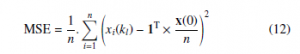
Here, k_l is the label of the iteration when the algorithm is completed at each vertex. The other metric, i.e., the number of the iterations, is applied in order to identify how long the algorithm has to be executed until the consensus upon the sum of all the initial inner states is achieved.

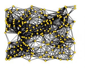
Figure 2: Representative of generated RGGs

4. Experiments and Discussion

In this section, we present the results obtained in Matlab2016a and Matlab2018b and discuss the character of the depicted functions and observable phenomena.

In the first experiment, we analyze the precision of the final estimates quantified by MSE when AC is bounded by the stopping criterion presented in [13]. As already mentioned, we examine two scenarios: either the initial states (i.e., before AC begins – referred to as scenario 1) or the final estimates (i.e., after AC is completed

– referred to as scenario 2) are multiplied by the network size n. From the results shown in Figure 3 and 4, we can observe in both examined scenarios that a decrease in the value of accuracy (see (a), (b), (c), and (d) in both figures for the results achieved for diffent values of accuracy) and an increase in the value of counter threshold ensure that MSE is smaller for each analyzed mixing parameter . Moreover, it can be seen that also an increase in the value of the mixing parameter  results in a decrease in MSE for each accuracy and counter threshold. Furthermore, in scenario 2, we can see that

Figure 3: MSE [dB] averaged over 30 dense RGGs – fully-distributed approach is implemented, initial inner states are multiplied by network size

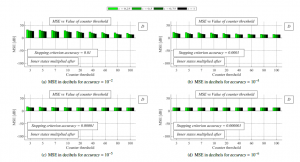
Figure 4: MSE [dB] averaged over 30 dense RGGs – fully-distributed approach is implemented, final estimates are multiplied by network size the precision of the final estimates is much smaller than in scenario 1, and a decrease in accuracy (see (a), (b), (c), and (d)) and an increase in counter threshold have a significantly smaller impact on an increase in the precision compared to scenario 1.

In the next experiment, we analyze the convergence rate expressed as the number of the iterations for the consensus achievement in both scenarios again. From the presented results in Figure 5 and 6, it can be seen that a decrease in the values of accuracy (see (a), (b), (c), and (d)) and an increase in the values of counter threshold result in a deceleration of the algorithm (i.e., AC requires more iterations to be completed) for each examined mixing parameter  in both analyzed scenarios. Again, it is seen that AC with a larger mixing parameter  achieves a higher performace like in the previous analyzes. However, unlike the previous analysis, AC in scenario 2 outperforms AC in scenario 1 for each value of both accuracy and counter threshold, and therefore, mutliplying the initial states with the network size n ensures higher precision of the final estimates, but a higher convergence rate is achieved in scenario 2.

In the last experiment, we test AC with the centralized stopping criterion from [6]. In Figure 7 and 8, we depict MSE and the convergence rate expressed as the number of the iteration for the consensus for same accuracy as in the previous two experiments. From Figure 7, it can be observed that a decrease in accuracy (see (a), (b), (c), and (d)) results in a decrease in MSE, and so, the precision of the final estimates is increased. Compared to the analysed fully-distributed approach, we can see that the value of the mixing parameter  has only a marginal impact on MSE regardless of accuracy of the stopping criterion (in fact, increasing  ensures a small increase in the performace). Regarding the convergence rate, a higher value of the mixing parameter  ensures a higher convergence rate just like in the previous analyzes. Also, it is seen that a decrease in accuracy (see (a), (b), (c), and (d)) results in a lower convergence rate; therefore, more iterations are necessary for AC to be completed.

In the two following paragraphs, we turn our attention to a comparison of the centralized and the fully-distributed stopping criterion, which are analyzed in the previous parts – in all the comparisons, the results achieved for  = 1 are examined (i.e., the results achieved by the best performing initial configuration). From Figure 3, Figure 4, and Figure 7, where the precision of the final estimates is analyzed, we can see that a decrease in accuracy (see (a), (b), (c), and (d)) results in a decrease in MSE in all three cases. Also, it is seen that the value of the mixing parameter  has only a marginal impact on MSE when the centralized stopping criterion is applied in contrast to the fully-distributed approach. In addition, in Figure 4, it is seen that the value of the mixing parameter  less affects the precision of the final estimates for lower values of accuracy and higher values of counter threshold. Furthermore, in the first case, when AC is bounded by the fully-distributed stopping criterion in scenario 1, MSE is from the range <-97.12 dB – 9.63 dB>, meanwhile, in scenario 2, MSE takes the values from this interval <12.95 dB – 26.67 dB>. In the third case, when the centralized stopping criterion is implemented, the values of MSE are from <-131.80 dB – -52.07 dB>. Therefore, the centralized stopping criterion significantly outperforms the fully-distributed approach in terms of the estimation precision. Even though this approach achieves a significantly higher performance according to the MSE-metric, it is less appropriate for real-life implementations since it requires time-variant global information – the maximum and the minimum from all the current inner states at each iteration. In terms of the convergence rate expressed as the number of

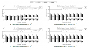
Figure 5: Convergence rate averaged over 30 dense RGGs – fully-distributed approach is implemented, initial inner states are multiplied by network size

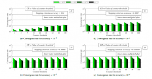
Figure 6: Convergence rate averaged over 30 dense RGGs – fully-distributed approach is implemented, final estimates are multiplied by network size

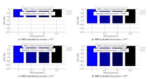
Figure 7: MSE [dB] averaged over 30 dense RGGs – centralized approach is implemented

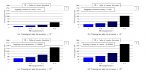
Figure 8: Convergence rate averaged over 30 dense RGGs – centralized approach is implemented

the iterations necessary for the consensus achievement (the results from Figure 5, Figure 6, and Figure 8 are compared), we can see that a decrease in accuracy (whereby a higher precision is achieved – see (a), (b), (c), and (d)) causes a deceleration of the algorithm in all three cases again. In the case, when AC is bounded by the fully-distributed stopping criterion in scenario 1, the convergence rate is from <121 – 560.4>. In scenario 2, the convergence is from the following interval <12.63 – 383.1>, and, in the third case, when the centralized stopping criterion is implemented, the convergence rate takes the following values <105.9 – 408.50>. So, it is seen that the highest convergence rate is achieved by the fully-distributed stopping criterion when the final estimates are multiplied by the network size n.

5. Conclusion

In this paper, we address AC for distributed summing whose execution is bounded by either a centralized or a fully-distributed stopping criterion. The results from our experiments show that decreasing accuracy ensures a higher precision of the final estimates but at a cost of a deceleration of the algorithm regardless of the applied stopping criterion. The precision of the final estimates can be improved also by increasing counter threshold when the fullydistributed stopping criterion is implemented. Moreover, it is proven that an increase in the mixing parameter  optimizes the algorithm in terms of both the precision and the convergence when AC is bounded by the fully-distributed stopping criterion. In the case of the implementation of the centralized one, the value of  has only a marginal impact on the precision of the final estimates, however, its higher values ensure a higher convergence rate like in the case of the fully-distributed stopping criterion. The fully-distributed stopping criterion achieves a higher precision when the initial inner states are multiplied by the network size n instead of the final estimates. However, on the other hand, multiplying the final estimates with n results in a higher convergence rate. Furthermore, it is proven that the centralized stopping criterion achieves higher performance in terms of the precision, however, this approach is less suitable for real-life implementations because it requires the information about the maximum and the minimum from all the current inner states at each iteration for its proper operating. The fastest is AC with the fully-distributed stopping criterion when the final estimates are multiplied by the network size n. On the other hand, in this case, the precision of the final estimates is significantly lower.

Acknowledgment

This work was supported by the VEGA agency under the contract No. 2/0155/19 and by COST: Improving Applicability of Nature Inspired Optimisation by Joining Theory and Practice (ImAppNIO) CA 15140. Since 2019, Martin Kenyeres has been a holder of the Stefan Schwarz Supporting Fund.

1.  M. Kenyeres, J. Kenyeres, I. Budinska, “Distributed linear summing in wire- less sensor networks” in IEEE 17th World Symposium on Applied Ma- chine Intelligence and Informatics (SAMI 2019), Herlany, Slovakia, 2019. https://doi.org/10.1109/SAMI.2019.8782782
2. H. Yetgin, K. T. K. Cheung, M. El-Hajjar, L. Hanzo, “A sur- vey of network lifetime maximization techniques in wireless sen- sor networkss” IEEE Commun. Surv. Tutor., 19(2), 828–854, 2017. https://doi.org/10.1109/COMST.2017.2650979
3.  B. Rashid, M. H. Rehnami, “Applications of wireless sensor networks for urban areas: a survey” J. Netw. Comput. Appl., 60, 192–219, 2016. https://doi.org/10.1016/j.jnca.2015.09.008
4. T. Qiu, A. Zhao, F. Xia, W. Si, D. O. Wu, “ROSE: robustness strategy for scale- free wireless sensor networks” IEEE/ACM Trans. Netw., 25(5), 2944–2959, 2017. https://doi.org/10.1109/TNET.2017.2713530
5. B. Krishnamachari, D. Estrin, S. B. Wicker, “The impact of data aggrega- tion in wireless sensor networks” in 22nd International Conference on Dis- tributed Computing Systems Workshops (ICDCSW 2002), Vienna, Austria, 2002. https://doi.org/10.1109/ICDCSW.2002.1030829
6. M. Kenyeres, J. Kenyeres, V. Skorpil, “The distributed convergence clas- sifier using the finite difference” Radioengineering, 25(1), 148–155, 2016. https://doi.org/10.13164/re.2016.0148
7. Y. Liu, M. Dong, K. Ota, A. Liu, “ActiveTrust: secure and trustable routing in wireless sensor networks” IEEE Trans. Inf. Forensics Secur., 11(9), 2013–2027, 2016. https://doi.org/10.1109/TIFS.2016.2570740
8. D. Izadi, J. H. Abawajy, S. Ghanavati, T. Herawan, “A data fusion method in wireless sensor networks,” Sensors, 15(2), 2964–2979, 2015. https://doi.org/10.3390/s150202964
9.  L. Xiao, S. Boyd, S. Lall, “A scheme for robust distributed sensor fusion based on average consensus” in 4th International Symposium on Information Processing in Sensor Networks (IPSN 2005), Los Angeles, CA, USA, 2005.
10.  G. Stamatescu, I. Stamatescu, D. Popescu, “Consensus-based data aggregation for wireless sensor networks” Control. Eng. App. Inf., 19(2), 43–50, 2017.
11.  A. K. Idrees, W. L. Al-Yassen, M. A. Taam, O. Zahwe, “Distributed data aggregation based modified K-means technique for energy conservation in periodic wireless sensor networks” in 2018 IEEE Middle East and North Africa Communications Conference (MENACOMM 2018), Jounieh, Lebanon, 2018. https://doi.org/10.1109/MENACOMM.2018.8371007
12.  Q. Chen, H. Gao, Z. Cai, L. Cheng, J. Li, “Distributed low-latency data ag- gregation for duty-cycle wireless sensor networks” IEEE/ACM Trans. Netw., 26(5), 2347–2360, 2018. https://doi.org/10.1109/TNET.2018.2868943
13.  M. Kenyeres, J. Kenyeres, M. Rupp, P. Farkas, “WSN implementation of the average consensus algorithm” in 17th European Wireless Conference 2011 (EW 2011), Vienna, Austria, 2011.
14.  D. Merezeanu, M. Nicolae, “Consensus control of discrete-time mul- tiagent systems,” U. Politeh. Buch. Ser. A, 79(1), 167–174, 2017. https://doi.org/10.1109/TNET.2018.2868943
15.  P. Jesus, C. Baquero, P. S. Almeida, “A survey of distributed data ag- gregation algorithms” IEEE Commun. Surv. Tutor., 17(1), 381–404, 2015. https://doi.org/10.1109/COMST.2014.2354398
16. A. Olshevsky, “Linear time average consensus and distributed optimiza- tion on fixed graphs” SIAM J. Control. Optim., 55(6), 3990–4014, 2017. https://doi.org/10.1137/16M1076629
17.  G. Oliva, R. Setola, C. N. Hadjicostis, “Distributed finite-time average- consensus with limited computational and storage capability” IEEE Trans. Con- trol. Netw. Syst., 4(2), 380–391, 2017. https://doi.org/10.1137/16M1076629
18. L. Faramondi, R. Setola, G. Oliva, “Performance and robustness of discrete and finite time average consensus algorithms” Int. J. Syst. Sci., 49(12), 2704–2724, 2018. https://doi.org/10.1080/00207721.2018.1510059
19.  J. Gutierrez-Gutierrez, M. Zarraga-Rodriguez, X. Insausti, “Analysis of known linear distributed average consensus algorithms on cycles and paths” Sensors, 18(4), 1–25, 2018. https://doi.org/10.3390/s18040968
20. T. C. Aysal, B. N. Oreshkin, M. J. Coates, “Accelerated distributed average consensus via localized node state prediction” IEEE Trans. Signal Process., 57(4), 1563–1576, 2009. https://doi.org/10.1109/TSP.2008.2010376
21.  V. Schwarz, G. Hannak, G. Matz, “On the convergence of average consensus with generalized Metropolis-Hasting weights” in 2014 IEEE International Con- ference on Acoustics, Speech, and Signal Processing (ICASSP 2014), Florence,
    Italy, 2014. https://doi.org/10.1109/ICASSP.2014.6854643
22.  L. Xiao, S. Boyd, “Fast linear iterations for distributed averaging” Syst. Control.
    Lett., 53(1), 65–78, 2004. https://doi.org/10.1016/j.sysconle.2004.02.022
23.  N. E. Manitara, C. N. Hadjicostis, “Distributed stopping for aver- age consensus in directed graphs via a randomized event-triggered strategy” in 6th International Symposium on Communications, Con- trol and Signal Processing (ISCCSP 2014), Athens, Greece, 2014. https://doi.org/10.1109/ISCCSP.2014.6877918
24.  S. V. Macua, C. M. Leon, J. S. Romero, S. S. Pereira, J. Zazo, A. Pages-Zamora,
    R. Lopez-Valcarce, S. Zazo, “How to implement doubly-stochastic matrices for consensus-based distributed algorithms” in 2014 IEEE 8th Sensor Array and Multichannel Signal Processing Workshop (SAM 2014), A Coruna, Spain, 2014. https://doi.org/10.1109/SAM.2014.6882409
25.  V. Schwarz, G. Matz, “Nonlinear average consensus based on weight morphing” in IEEE International Conference on Acoustics, Speech, and Signal Processing (ICASSP 2012), Kyoto, Japan, 2012. https://doi.org/10.1109/ICASSP.2012.6288578
26.  S. S. Pereira, A. Pages-Zamora, “Mean square convergence of consensus al- gorithms in random WSNs” EEE Trans. Signal Process., 58(5), 2866–2874, 2010. https://doi.org/10.1109 3140

(Click Here)

(Click Here)