1. Introduction

Given RL properties, a growing interest was developing these last years in order to extend reinforcement learning to multiagent systems (MASs). MASs are applied to a wide variety of domains including robotic teams [4, 5], air traffic management [6] and product delivery [7].

We are specifically interested in distributed cooperative mobile robots, Where multiple cooperative robots can perform tasks faster and more efficiently than a single robot. The decentralized point of view provides many potential benefits interests (e.g., the same reward function), thus the increase in individual’s benefit also leads to the increase of the benefits of the whole group[10, 11].

In recent years, an increasing number of researches have shown interest in extending reinforcement learning (RL) to MASs in the powerful framework of Markov games (MG, also known as stochastic games, SG), and many promising multiagent reinforcement learning (MARL) algorithms have been proposed [10][12]-[13]. These methods can be divided into two big categories: the case of independent learners (ILs) where each agent only knows its own actions [13] and the case of joint actions learners (JALs) where each agent collects information about their own choice of action as well as the choices of other agents [14].

Many algorithms derived from these both IALs and JALs can learn the coordinated optimal joint behaviors and provide certain convergence guarantees as well but in simple cooperative games (matrix games, few players, not fully stochastic environment, etc). However, they fail when the domain becomes more complex [15, 16], especially when the number of agents or state spaces increases, resulting in large memory requirement, slowness in learning speed and then more challenging coordination.

As JALs offer good coordination results but suffer from the curse of dimensionality, a new kind of distributed multi-agent reinforcement learning algorithm, called the ThMLA-JAG (Three Model Learning Architecture based on Joint Action Generalization) method, is proposed here. The main idea is to decompose the coordination of all JALs into several twoagent coordinations. Validation tests which are realized on a pursuit problem show that an overall coordination of the multi-agent system is ensured by the new method as well as a great reduction of the amount of information managed by each learner, which considerably accelerates the learning process.

To the best of our knowledge, this is the first distributed MARL system that decompose the multi-agents learning process into several two-agents learning systems. The system is decentralized in the sense that learned parameters are split among the agents: each agent learns by interacting with its environment and observing the results of all agents’ displacements. Hence no direct communication is required into learning agents, a communication that can be expensive or insufficient because of bad synchronization and/or limited communication range [17]. As such, the proposed approach is different from methods that learn when such communication is necessary [9][18]-[19]. We particularly show that the system remains effective even when agents’ information are distorted due to frequent environmental changes.

The rest of the paper is arranged as follows. In section 2, we introduce some basic reinforcement learning concepts. In section 3, two existing RL methods on which our proposed approach is based are presented. Section 4 is dedicated to present the ThMLA-JAG method. Several experiences are conducted in section 5 showing the efficiency of our proposals. Some concluding remarks and future works are discussed in section 6.

2. Reinforcement learning

Markov Decision Processes (MDPs) are often used to model single-agent problems. MDPs [20] are suitable for studying a wide range of optimization problems that have been solved by dynamic programming and reinforcement learning. They are used to model scenarios where an agent has to determine how to behave based on the current state’s observation. More precisely, a Markov model is defined as a 4-tuple

(S,A,T,R), where S is a discrete set of environmental states, A is a discrete set of agent actions, R : S×A → < is a reward function and T : S × A → Π(S) is a state transition function ( Π(S) is a probability distribution over S). We write T(s,a,s⁰) as the probability of making a transition from s to s⁰ taking action a. The action-value function Q^∗(s,a) is defined as the expected infinite discounted sum of rewards that the agent will gain if it chooses the action a in the state s and follows the optimal policy. Given Q^∗(s,a) for all state/action pairs, the optimal policy π^∗ will be developed as the mapping from states to actions such that the future reward is maximized [1].

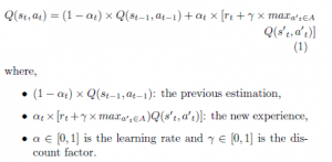
One of the most relevant advances in reinforcement learning was the development of the Qlearning algorithm, an offpolicy TD (temporal-difference) control algorithm [15, 21]. Q-learning is especially used when the model (T and R) are unknown. It directly maps states to actions by using a Q function updated as in (1):

Despite its multiple successful results in single agent cases, Qlearning can’t be directly applied to multi-agent systems. In fact, learning becomes a much more complex task when moving from a single agent to a multi-agent setting. One problem is the lack of the single agent framework’s convergence hypotheses. For instance, the environment is no longer static from a single-agent perspective due to many agents working on it: this is a commonly cited source of multi-agent learning systems difficulties [22]. Another issue is the communication between agents: How to ensure a relevent information exchange for effective learning [23]?, and finally the problem of multi-agent coordination in order to ensure a coherent joint behavior.

In what follows, several MAL methods derived from Qlearning are presented and classified according to the state/action definition.

2.1         Individual state / individual action

Many researchers are interested on extending Qlearning to distributed MAS using cooperative ILs. They aim to design multiple agents capable of performing tasks faster and more reliably than a single agent. Examples include PA (Policy Averaging) [24], EC (Experience Counting) [25], D-DCM-MultiQ (Distributed Dynamic Correlation Matrix based MultiQ) [17], CMRL-MRMT (Cooperative Multi-agent learning approach based on the Most Recently Modified Transitions) [26] and CBG-LRVS [27]. Here, each entry of the Qfunction is relative to the individual state/action pair of the agent itself like in the case of single-agent learning and a direct communication is used to share information between different learners. These methods use also the assumption that all learners can be in the same state at the same time which eliminates the coordination problem. So, these methods succeed to establish a cooperative learning but become inapplicable when considering the collision between learners, like the case in reality of mobile and autonomous robotic systems.

2.2         Joint state / individual action

To better address the coordination problem, many other learning algorithms have been proposed in literature while keeping collisions between learners, like, decentralized Qlearning [23], distributed Qlearning [15], WoLF PHC [22], Implicit coordination [28], Recursive FMQ [16] and Hysteritic learners

[29].

In such methods, agents are fully cooperative which means that they all receive the same reward and are noncommunicative that are unable to observe the actions of other agents. These methods are based on Markov games, i.e, each learner updates its Qvalues using joint states ( relatives to all agents and even other elements presenting in the environment) and individual actions ( specific to the agent itself). Their performances can greatly vary between successful and unsuccessful coordination of agents.

As explained in [13], no one of those algorithms fully resolves the coordination problem. Complications arise from the need of balance between exploration and exploitation to ensure efficiency like in single RL algorithms. But the exploration of an agent induces noise in received rewards of the group and can destabilize the learned policies of other ILs.

To sort out this problem, called the alter-exploration problem, many parameters, which the convergence relies on, are introduced. So, the main drawbacks of these methods are that parameter tuning is difficult and that when the number of agent increases, the difficulty of coordination increases and the alter-exploration problem outweighs. The learning velocity is also highly affected when altering the number of agents and/or the environment size due to the use of joint states.

2.3         Joint state / joint action

Given ILs’ limitations, methods using JALs are much more used for stochastic games[14]. They can provide distributed learning while avoiding collisions between agents. They solve ILs’ problems since the whole system’s state is considered by each learner, i.e, the Qvalues are updated using joint states and joint actions. However, JALs suffer from combinatorial explosion of the size of the state-action space with the number of agents, as the value of joint actions is learnt by each agent, contrary to ILs that ensure a state space size independent of the number of agents.

As an example, TM-LM-ASM (team-mate model- learning model- Action Selection Model) [30] is a JAL method that combines traditional Q-learning with a team-mate modeling mechanism. To do that, each learner has to memorize a table Q storing all possible joint states/actions pairs and a table P storing all possible joint states/actions pairs except its own action. The Q table is used by the learning model as similar as the Qlearning method and the P table is used by the teammate model to estimate the behaviors strategies of other agents. Then, the strategy used by the learner to select an action is done by the action selection module using both the P and Q tables.

Experiments done on a pursuit game [30] using two predators and one moving prey show the effectiveness of the TMLM-ASM method and that it ensures a global coordination without the need of a direct communication between different members. However, obtained results are limited to two-agent systems. A problem of state space explosion can be obviously detected when increasing the number of agents because of the use of joint states and joint actions. As an example, let’s consider the case of N_agents agents able to execute N_actions actions in an L × L grid world. If the state of every agent is relative to its position in the grid, every learner has to store a table Q containing ( entries and a table P having  entries, without forgetting the significant number of possible team-mates actions’ combinations to consider when updating the table P and when choosing the next action to execute, that’s:  possible actions’ combinations.

If we examine the case of 4 agents which can make 5 actions in a 10 × 10 grid world, we obtain:

• 625 · 10⁸ entries of the table Q,
• 125 · 10⁸ entries of the table P,
• 125 possible combinations of team-mates’ actions in every state.

As it is mentioned in the theoretical convergence of the Qlearning algorithm [15], an optimal policy is only achieved if every state action pair has often been performed infinitely. For the above described example, we can see that a first visit of each state/action pair isn’t obvious and requires a long time. The amount of memory needed for storing the tables P and Q is also significant. A huge computing power is thus required so that all possible combinations of team-mates’ actions can be taken into account and this is at every learning step (during the updates of P and Q and when choosing actions).

2.4         Learning by pair of agents

To solve the state space explosion problem along with ensuring a satisfactory multi-agent coordination, Lawson and Mairesse [18] propose a new method inspired by both ILs and JALs approaches. The main idea is to learn a joint Q-function of two agents and to generalize it to any number of agents. Considering a system of N_agents agents, at any learning step, each agent has to communicate with its (N_agents − 1) teammate agents, update its (N_agents − 1) Q tables of two agents and then identify the next joint action to follow. Note that the same joint action must be chosen by all the learners. Additional computations are then required. Indeed, the most promising joint action is not directly determined from a joint table Q, as in the case of joint actions learners, but it needs the evaluation of the sum of (N_agents − 1) values of Q. Also, (N_agents − 1) updates of Q are done instead of one update of the joint table. However, this increase in required computing power is widely compensated by the advantages that present this method compared with the approaches using ILs or JALs, namely:

• By learning through agents’ pairs as the JAG method, a huge reduction in the number of state/action pairs is ensured which leads to the acceleration of the system convergence. As illustrated in Table 1, these memory savings widen with the increase of the environment size and/or the number of agents.
• Contrary to independent agents, a global coordination is provided by the JAG method because this method evaluates all possible joint actions of every pair of agents and chooses the global joint action (of the whole multi-agent system) after maximizing the Qvalue of each of these pairs. This is based on the assumption that a global coordination is ensured by coordinating each couple of agents, provided that the policy obtained for two agents is optimal.

Several experiences are made by Lawson and Mairesse [18] on the problem of the navigation of a group of agents in a discrete and dynamic environment so that each of them reaches its destination as quickly as possible while avoiding obstacles and other agents. The results of these experiences confirm the aforesaid advantages, namely an acceleration of learning with a global coordination as in the case of JALs.

However, the distribution of learning does not facilitate the task but results in an identical treatment of the same information by all the agents. More precisely, in every iteration, agents communicate their new states and rewards to all their team-mates. As a consequence, each of them updates the Qentries of all agents’ couples and executes the JAG procedure to choose the next joint action. Another communication is then necessary to make sure that the same joint action is chosen by all learners. Thus, the JAG method seems to be less expensive by adopting a centralized architecture: only one agent is responsible for updating information and for choosing actions and informs other agents of their corresponding actions. Conversely, every agent executes its own action and informs the central entity of its new state and the resulted reward.

3. Proposed reinforcement learning algorithm

As explained earlier, the JAG method [18] ensures a global coordination while using independent learners but needs a centralized process to make sure that all agents choose the same joint action at each learning step, whereas the TM-LM-ASM method [30] is a full distributed learning approach that also provides a global coordination but employs joint action learners which make it unsuitable for systems considering many agents and/or large state spaces.

Our objective is to develop a new intermediate approach between TM-LM-ASM and JAG. The main idea is to generalize the TM-LM-ASM architecture which is learned by two agents to a larger number of agents while using the JAG decomposition instead of joint state-action pairs. The new proposed approach is called ThMLA-JAG (a Three-Model Learning Architecture using Joint Action Generalization).

According to the ThMLA-JAG method, the multi-agent coordination process is divided into several two-agents learning tasks. Assuming that the system contains N_agents agents, each agent must memorize (N_agents − 1) P-Tables of two agents for the team-mates’ model and (N_agents −1) Q-Tables of two agents for the learning model.

3.1         The team-mates’ model

Consider a system of N learning agents in a joint state s = (s₁,…,s_Nagents). At a learning step t, a learning agent i under consideration executes an action and observes its partners’ actions (), the new obtained state) and the resulted reward r. Then, it updates (N_agents − 1) P-tables concerning each partner j for each action a_j that can be tried by this agent j in the experimented state s = (s_i,s_j). The table P_ij concerning the pair of agents (i,j) can be updated using (2), similarly to the TM-LM-ASM method when is applied to two-agent systems.

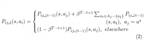
where, β ∈ [0,1] is the learning rate that determines the effect of previous action distribution, and T is the number of iterations needed for the task completion. s and s⁰ are joint states that present the instantaneous positions of agents (i,j) in the environment.

3.2         The learning model

Similar to the JAG method, (N_agents − 1) updates are made by each learner at each learning step. Each update concerns an entry of one of the (N_agents − 1) Q-tables that are saved by this learner and is relative to one of its partner.

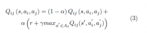
If we consider that the transition ( had been executed by a learner i while another learner j executed the transition (s_j,a_j) → s⁰_j, the table Q_ij corresponding to the pair (i,j) with the joint state s = (s_i,s_j) and the joint action a = (a_i,a_j) can be updated using (3), as when applying the TM-LM-ASM method for two agents.

Table 1: Comparison of the Q size following the joint and the JAG method. Note that Nagents agents evolve in an L × L grid world by executing Nactions possible actions and the state of each agent corresponds to its position in the grid Nagents Nactions L Size of Q using TM-LM-ASM the JAG method Size of Q for two agents Total size of all agents’ Q N A L (L2 × A)N (L2 × A)2 (L2 × A)(N−1) 4 4 5 10 50 108 2.56 · 1010 1016 104 1.6 · 105 108 6 · 104 9.6 · 105 6 · 108 8 4 5 10 1016 6.5536 · 1020 104 1.6 · 105 28 · 104 44.8 · 105 50 1032 108 28 · 108

where,

Thus, the team-mate model is exploited by the learning model. More precisely, the best move in the next state s⁰ relies on the next action  of the agent i under consideration and the next action  of its partner j. Given that the Q function of this later isn’t known by agent i, a prediction of its action is done using the memorized team-mate model. For the examined agent, the action that should be preferably executed in the next state is determined by the exploitation of its Q function.

3.3         The action selection model

For a better selection of the next action to execute, a generalization of the action selection model proposed by Zhou and Shen [30] for 2 agents to N agents (N >= 2) is possible by exploiting all stored P-tables and Q-tables of the learner. To this end, for each agent i having (N_agents−1) team-mates and staying at a joint state s = (s1,…,s_i,…,s_Nagents), the action  to be executed in that state s can be selected by using (4):

where, () are predicted by agent i as the next actions to be executed by its partners in the joint state s, A_i is the set of possible actions of agent i and

) is the conditional expectation value of action a^∗_i of agent i when it considers the team-mates’ model:

For all ) is calculated using (5):

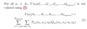
where, (s_i,s_j) is the actual state of agent i and its team-mate j and A_j is the set of all possible actions of agent j. Here, all possible actions of team-mates are equally considered and there’s no prediction of any particular joint action. This can be explained by the fact that, for each pair of agents (i,j), P_ij and Q_ij have initially the same values for all state/action pairs. As the learning progresses or new circumstances take place (such as collisions or environmental changes), a particular set of state/action pairs will become favoured as a result of the increase of their corresponding P_ij and Q_ij values. Therefore, different values V will be attributed to each action a_i of agent i. Then, a greedy choice following (4), allows the agent i to select the most promising action a^∗_i in the current state

s.

3.4         Improving multi-agent coordination

When updating a table Q_ij related to the team-mate j, the learner i has to predict the most promising joint action ( in the next state. As described in (3), its own action is that maximizing Q_ij in that state. However, our proposition assumes that each agent has (N_agents −1) Q-tables corresponding to its (N_agents −1) partners and all these Q-tables will be exploited during the choice of the action to be really executed. Thus, by referring to the unique table Q_ij when predicting a possible next action, the predicted action will not necessary reflect the one which will be really experimented in the next state. As a result, the learner can continuously oscillate between two consecutive states if those states are updated according to a predicted state different from that really visited. For that, it would be better to predict the action maximizing the next state using the maximum amount of information, explicitly, all the Q-tables and P-tables which have been stored by the learner. Thus, the updated version of (3) is shown by

where, a^∗_j is identified as before in (4) and a^∗_i is calculated using the predefined action selection model of (4): it is the same strategy used for real actions’ selection. This modification in the update of the Q-function will be further justified in the experimental section.

3.5         The proposed learning algorithm

A possible extension of the algorithm proposed by Lawson and Mairesse [18] for a system having more than two agents is presented by algorithm 1 and illustrated in Figure 1. Note that all agents are learning synchronously, specifically:

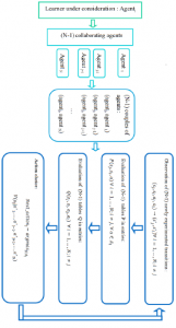
Figure 1: The ThMLA-JAG learning architecture

• Initialize learning (the steps 1,…,14 of algorithm 1),

• Select the action, execute it and observe the result (the steps 17,…,20 of algorithm 1),
• Update P-table (the step 22 of algorithm 1),
• Update Q-table (the step 23 of algorithm 1). Two alternatives of updating a Q-table will be compared in the experimental section: (3) and (6),
• Test the end of learning or the release of a new episode (the steps 25 and 26 of algorithm 1),
• Go to a new iteration in the same episode (the steps 27 and 28 of algorithm 1).

It should also be noted that the reward is defined by pair of agents in accordance with the learning architecture, i.e, every two agents receive a specific reward that describes the result of their own displacement. In what follows, we are going to examine two test cases:

• In the first case (S1: a temporary dynamic environment), the prey is temporary moving and each predator should be able to build an optimal path from its starting position to that target while avoiding obstacles, other predators and the prey as well as to correct this path after each environmental change. An episode ends if the prey is captured or that it exceeds 1000 iterations. Initially, the environment is in the form of Figure 2. After 1200 episodes, the prey moves to a new position as shown in Figure 2-b.

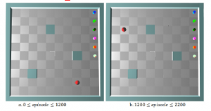
Figure 2: The testing environment of S1

Figure 3 describes the environment used to test this scenario. Once an episode is ended, agents are relocated on the right extremity of the labyrinth and a new trial begins. Because collisions between agents aren’t permitted and in order to test a system containing more than four agents, we suppose that the prey is captured if each hunter is in one of its eight neighboring cells including corners. Figure 3-a describes a possible capture position.

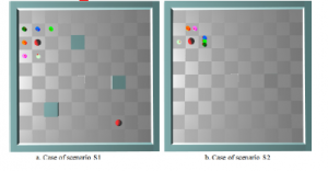
Figure 3: Example of capture position

Algorithm 1 Algorithm ThMLA-JAG Require: N: the total number of agents S = {(si,sj);i,j = 1…N} is the set of possible states for all agents’ pairs (i,j) Ai is the set of possible actions of agent i Ensure: for agent: i = 1…N do for team − matei : j = 1…N, j 6= i do for s = (si,sj) ∈ S × S do for a = (ai,aj) ∈ Ai × Aj do Q end for end for end for end for while learning in progress do for agent i = 1…N do t ← 0, initialize its own current state si,t end for for each learning step do for agent i = 1…N do Observe the current joint state st = (s1,t,s2,t,…,sN,t) Choose an action ai,t following equation(4) Execute ai,t and observe the actions being simultaneously executed by other team-mates for team − matei : j = 1…N, j 6= i do Determine the new state st+1 = (si,t+1,sj,t+1) and the corresponding reward rt+1 = rij Update Pij(si,t,sj,t,aj) following equation (2),for all aj ∈ Aj Update Qij(si,t,sj,t,ai,t,aj,t) following equation (3) or equation (6) , where aj,t is the simultaneous action of

• In the second case ( S2: a highly dynamic environment), agents move in a frequently dynamic environment and agent j

end for

if the new state s_t+1 is the goal state then

The episode is ended, go to 11 else {s_t+1 6= goal state} t ← t + 1, go to 15 end if end for

end for

end while

devoid of obstacles. At each stage of learning, the prey has a probability equal to 0.2 to remain motionless or to move towards vertically or horizontally neighboring cells. As to hunters, they can share the same position except the one containing the prey. These agents are initially in random positions. They move according to 5 above-mentioned actions in a synchronized way until they catch the prey or their current episode exceeds 1000 iterations. Once an episode is ended, these agents are relocated at new random positions and a new episode begins. The prey is captured when all hunters are positioned in the vertically and/or horizontally neighboring cells of that prey.

In the rest of the paper, the term agent refers to only a predator (a learner). Some experiences are conducted while varying the number of agents. The results reported below are obtained by average results of 30 experiments where each one contains 2200 episodes.

3.6         Communication between agents

Communication between the different agents must be ensured by an autonomous multi-agent network system which aims to exchange data between the different nodes while meeting and maintaining certain communication performance requirements(coordination, synchronization of messages and cooperation). As wireless technology has led to consider a new era for robotics, where robots are networked and work in cooperation with sensors and actuators, we have defined a wireless communication allowing the different agents to work in cooperation, and to exchange data locally in a multi-agent system.

A wireless access point is used to operate in the command link of a mobile agent. The link will carry data signals for the other agents.

3.7         Parameter setting

As most RL methods, the major problems met during the implementation of the ThMLA-JAG algorithm (algorithm 1) are essentially the initialization of its parameters. To do it, several values had been experimented and the best configuration was then adopted to test the above-mentioned test cases. As a result, the same distribution of rewards is used in both scenarios, namely:

• a penalty of 0.9 is attributed to every agent striking an obstacle and/or to every couple of colliding agents,
• a reward of 3 is received by every couple of agents having captured the prey,
• a reward of -0.05 is given to every agent moving to a new state without neither colliding nor capturing the prey.

Concerning the other parameters, they are initialized as follows:

• the learning rates α = 0.8 and β = 0.8,
• the update factor γ = 0.9,
• the Qvalues (values of Q-table) are set to 0.04,
• the Pvalues (values of P-table) are set to 0.2,

Finally, the ThMLA-JAG method is tested in scenarios S1 and S2 while comparing both possibilities of update of the table Q, that are:

• according to (3) where the Qtable concerning one teammate is only updated according to the information saved by the current learner about this latter. In this case, the learning method to be tested is indicated by ThMLAJAG1,
• according to (6) where the Qtable concerning one teammate is updated according to all information saved by the current learner, including those concerning other team-mates. Here, the variant to be tested is denoted by ThMLA-JAG2.

3.8         Memory savings

According to the ThMLA-JAG method and regardless of the manner in which the Q-tables are updated, a lot of saving in memory is ensured comparing to the TM-LM-ASM method (a JAL method) as well as the Hysteritic Qlearning method (an IL method) and this is all the more important as the number of agents increases. Table 2 illustrates this result.

3.9         Computation savings

In addition to memory savings, important computation savings are provided by the ThMLA-JAG1 method and are described in Table 3. Note that a P_entry (respt. a Q_entry) designates an entry in the table P (respt. Q).

3.10        Comparing the two variants of ThMLA-JAG

In this section, we will compare ThMLA-JAG1 and ThMLAJAG2 using 4-agent systems in both test cases S1 and S2.

3.10.1      Testing S1

As noted by Figure 4 and Table 4, both ThMLA-JAG1 and ThMLA-JAG2 lead to the system convergence before and after the environmental change. Figure 4-a shows the number of iterations needed for each episode over time while Figure 4-b describes the number of collisions in each learning episode.

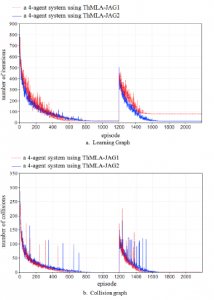
Figure 4: Testing the S1 scenario with a four-agent system (average of 30 experiences)

Table 2: Variation of the saved information’s size according to the adopted method and the number of learners (|S| = 361 and |A| = 5) Learning              NAgents Size of tables P        Size of tables Q method

We can see that in both environments, the agents succeed to catch the prey without colliding with each other or with obstacles and this is after some iterations (about 850 episodes in the first environmental form and 450 episodes after moving the target). On another hand, when updating a Q-table by only using the information of the corresponding team-mate (ThMLA-JAG1), the number of collisions is less than by exploiting the information of all other team-mates (ThMLA-JAG2). This is because with ThMLA-JAG2, the action resulting previous collisions is more likely to be chosen again, especially if these collisions concerned only some members of the multi-agent system.

On the contrary, the learning following ThMLA-JAG1 is much slower than that using ThMLA-JAG2. Figure 4-a and Table 4 show this result. Using ThMLA-JAG1, the first episodes are longer and the adaptation to the new environmental form requires more iterations than ThMLAJAG2. Moreover, after displacing the target, the agents following ThMLA-JAG1 risk to not find a path leading to the new position of the target. Some experiences considering the ThMLA-JAG1 method are ended without a successful adaptation to the new environmental form. This explains the reason why the average length of the constructed path is equal to 80 steps in case of ThMLA-JAG1 and only 12 steps with ThMLA-JAG2. Besides, by observing the curves of collisions of ThMLA-JAG1 (Figure 4-b), we notice the existence of few collisions even after the system convergence. These collisions are related to failed experiences.

The weakness of ThMLA-JAG1 is caused by the difference that can happen between the predicted action when updating the Qvalue and that will be really chosen using the adopted policy. This difference can block the learner between consecutive states. As the updates of Q no longer depend on recent movements, the Qvalues will remain invariants after some updates and the agent can’t modify or correct it.

3.10.2      Testing S2

The same remains true with the scenario S2. Figure 5 describes the number of captures done each 1000 episodes by considering two systems of 4 learning agents following ThMLA-JAG1 and ThMLA-JAG2, respectively. Results show that the number of captures after the system convergence are much more important and stable by considering ThMLA-JAG2: After 16 · 10⁴ iterations, the number of captures is slightly changing in the case of ThMLA-JAG2 due to the movement of the prey but is significantly degrading in the case of ThMLA-JAG1. This difference in learning performance lies in the fact that, with ThMLA-JAG2, the Q-update is more in line with the adopted PEE, contrary to ThMLAJAG1 where the system fails to converge to a final solution because the saved information can be considerably distorted by the movement of the prey which can occurs at every stage of learning.

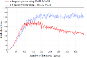
Figure 5: Variation of captures in function of the used learning method with the test case S2 (average of 30 experiences)

3.11        Effect of increasing the number of agents on the learning performance

In this section, we aim to evaluate the ThMLA-JAG2 method in both cases S1 and S2 while varying the number of agents from 2 to 6.

Table 3: Operations made by each learner at each learning iteration with |A| = 5 Operations Nagents TM-LM-ASM ThMLA-JAG1 ThMLA-JAG2 team-mate model Number of P-entries to update at each learning step N 2 4 |A|N−1 5 125 (N − 1) · |A| 5 15 (N − 1) · |A| 5 15 8 78125 35 35 Action selection Model Calculate V (ai) for every possible action ai of the current learner i by performing k sum of (Pentry · Qentry) where k N 2 4 8 |A|(N−1) 5 125 78125 (N − 1) · |A| 5 15 35 (N − 1) · |A| 5 15 35 Learning model Number of Q-entries to update at each learning step N 2 4 8 1 1 1 1 (N-1) 1 3 7 (N-1) 1 3 7 Number of P-entries to be browsed to predict the possible next action of all team-mates N 2 4 8 |A|N−1 5 125 78125 (N − 1) · |A| 5 15 35 (N − 1) · |A| 5 15 35 is equal to

3.11.1      Case of T1

From Figure 6, we can see that the multi-agent system converges to a near optimal and collision free path and this is regardless of the number of agents.

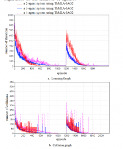
Figure 6: Effect of increasing the number of agents on the ThMLA-JAG2 method in the case of S1 (average of 30 experiences)

Likewise, agents succeed to adapt to the new environmental form once the prey is moved and the learning time isn’t considerably delayed by the addition of new agents as well. As shown by Table 5, the 4-agent system needs more episodes to converge than the 2-agent system but a smaller number of iterations and collisions. As for the 6-agent system, the learning is slightly slower than the other cases.

3.11.2      Case of S2

Promising results are also obtained in case of S2. Figure 7 shows the number of captures done each 1000 episodes by considering three systems containing 2, 4 and 6 agents and using the ThMLA-JAG2 method. The results prove that the learning is accelerated by adding new agents.

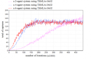
Figure 7: Variation of captures in function of the number of agents in the case of S2 (average of 30 experiences)

Table 4: Comparing ThMLA-JAG1 and ThMLA-JAG2 in the case of S1 with a four-agent system (average of 30 experiences) ThMLA- JAG1 ThMLA- JAG2 Total of iterations ∈ [0 − 800] 100596 94001 Total of collisions ∈ [0 − 800] 19080 22017 ∈ [1200 − 1850] 90144 52693 ∈ [1200 − 1850]                                                                                               10781                                   13541 Table 5: Impact of varying agents’ number on the performance of ThMLA-JAG2 in the case of S1 (average of 30 experiences) [0-1200] Episodes for convergence Iterations for convergence Total of collisions before convergence 583 114382 24776 850 94786 22051 1028 140343 43991 Total of collisions after convergence 0 0 0 [1200-2200] Episodes for convergence Iterations for convergence Total of collisions before convergence 1694 97795 21047 1658 50326 13533 1948 62682 23205 Total of collisions after convergence 0 0 0

• From the beginning of learning to the 15 · 10^4th iteration, the number of captures done each 1000 episodes increases over time and is all the more important as agents are more numerous.
• From the 15·10^4th to the 42·10^4th iteration, the number of captures further increases in case of 2-agent systems and converges to approximately 140 captures every 1000 episodes in the case of 4-agents and 6-agents systems with low oscillations due to the movements of the prey.

4. Conclusion

In this paper, we have studied the problem of cooperative learning with avoiding collisions between agents. For that, a new learning method, called ThMLA-JAG, has been proposed. Using this method, a global coordination is ensured between agents as well as a great reduction in the amount of stored information and the learning computations with regard to classic joint RL methods. This is effectively due to the decomposition of learning into pairs of agents. By this decomposition, the learning process is considerably accelerated and the problem of the states’ space explosion is partially resolved.

This research is still in its early stages. Experimental results so far point to the fact that the proposed method is a good alternative to RL algorithms when dealing with distributed decision making in cooperative multi-agent systems. However, all conducted tests on the ThMLA-JAG method are restricted to small environments with a limited number of agents. We expect to further improve our work by expanding it with the ability to solve more complex scenarios. Possible test cases include more agents, several targets, as well as continuous state spaces. Such complex elements typically describe real-world applications.

Furthermore, all agents in our current Markov game model can observe the global state space, while in reality this may not be feasible. More research into how agents can still efficiently collaborate when only partial state information is available would be worthwhile. In addition, the study of fully competitive MARL methods is also a good focus for next researches.

Acknowledgements

This research received no specific grant from any funding agency in the public, commercial or not-for-profit sectors.

1.  R. Sutton, A. Barto, Reinforcement Learning: An Introduction, IEEE Transactions on Neural Networks 9 (5) (1998) 1054–1054. doi:10.1109/TNN.1998.712192.
2.  W. Zemzem, M. Tagina, A New Approach for Reinforcement Learn- ing in non Stationary Environment Navigation Tasks, International Review on Computers and Software 7 (5) (2012) 134–143.
3.  W. Zemzem, M. Tagina, A novel exploration/exploitation policy accelerating learning in both stationary and non stationary envi- ronment navigation tasks, International Journal of Computer and Electrical Engineering 7 (3) (2015) 149–158.
4.  M. Wu, W.-H. Cao, J. Peng, J.-H. She, X. Chen, Balanced or multi-agent system for sim- gue of RoboCup, International Journal of Control, Automation and Systems 7 (6) (2009) 945–955. doi:10.1007/ s12555-009-0611-z.
5. L. Parker, C. Touzet, F. Fernandez, Techniques for learning in multi-robot teams, Robot Teams: From Diversity to Polymorphism. AK Peters.
6. K. Tumer, A. Agogino, Improving Air Traffic Management with a Learning Multiagent System, IEEE Intelligent Systems 24 (1) (2009) 18–21. doi:10.1109/MIS.2009.10.
7. S. Proper, P. Tadepalli, Solving multiagent assignment Markov de- cision processes, in: Proceedings of The 8th International Confer- ence on Autonomous Agents and Multiagent Systems, A.C.M, Bu- dapest, Hungary, 2009, pp. 681–688.
8. P. Stone, M. Veloso, Multiagent systems: a survey from a machine learning perspective, Autonomous Robots 8 (3) (2000) 345–383. doi:10.1023/A:1008942012299.
9.  Y. Cai, Intelligent Multi-robot Cooperation for Target Searching and Foraging Tasks in Completely Unknown Environments, Ph.D. thesis, University of Guelph (2013).
10.  C. Claus, C. Boutilier, The dynamics of reinforcement learning in cooperative multiagent systems, in: Proceedings of the National Conference on Artificial Intelligence, 1998, pp. 746–752.
11. X. Chen, G. Chen, W. Cao, M. Wu, Cooperative learning with joint state value approximation for multi-agent systems, Jour- nal of Control Theory and Applications 11 (2) (2013) 149–155. doi:10.1007/s11768-013-1141-z.
12.  J. Hao, D. Huang, Y. Cai, H.-f. Leung, The dynamics of reinforce- ment social learning in networked cooperative multiagent systems, Engineering Applications of Artificial Intelligence 58 (2017) 111– 122. doi:10.1016/J.ENGAPPAI.2016.11.008.
13.  M. Lauer, M. Riedmiller, Reinforcement Learning for Stochas- tic Cooperative Multi-Agent Systems, in: Ithe 3rd International Joint Conference on Autonomous Agents and Multi Agent systems, IEEE Computer Society, New York, USA, 2004, pp. 1516–1517. doi:10.1109/AAMAS.2004.226.
14.  L. Matignon, G. J. Laurent, N. Le, Independent reinforcement learners in cooperative Markov games: a survey regarding coor- dination problems, Knowledge Engineering Review 27 (1) (2012) 1–31. doi:10.1017/S026988891200057>.
15. E. Yang, D. Gu, Multiagent reinforcement learning for multi-robot systems: A survey, Tech. rep., 2004 (2004).
16.  C. Watkins, P. Dayan, Q-learning, Machine Learning 8 (1992) 279– 292.
17.  L. Matignon, G. Laurent, N. L. Fort-Piat, A study of FMQ heuristic in cooperative multi-agent games, in: In The 7th International Con- ference on Autonomous Agents and Multiagent Systems. Workshop 10: Multi-Agent Sequential Decision Making in Uncertain Multi- Agent Domains, aamas’ 08, Vol. 1, 2008, pp. 77–91.
18.  H. Guo, Y. Meng, Distributed Reinforcement Learning for Coordi- nate Multi-Robot Foraging, Journal of Intelligent and Robotic Sys- tems 60 (3-4) (2010) 531–551. doi:10.1007/s10846-010-9429-4.
19. J.-Y. Lawson, F. Mairesse, Apprentissage de la coordination dans les systèmes multi-agents, Master’s thesis, Catholic University of Louvain (2004).
20. W. Zemzem, M. Tagina, M. Tagina, Multi-agent Coordination us- ing Reinforcement Learning with a Relay Agent, in: Proceedings of the 19th International Conference on Enterprise Information Sys- tems, SCITEPRESS – Science and Technology Publications, 2017, pp. 537–545. doi:10.5220/0006327305370545.
21. M. L. Puterman, Markov Decision Processes: Discrete Stochas- tic Dynamic Programming (1994). doi:10.1080/00401706.1995. 10484354.
22. K. Tuyls, G. Weiss, Multiagent Learning: Basics, Challenges, and Prospects, AI Magazine 33 (3) (2012) 41. doi:10.1609/aimag. v33i3.2426.
23.  M. Bowling, M. Veloso, Multiagent learning using a variable learn- ing rate, Artificial Intelligence 136 (2) (2002) 215–250. doi:10. 1016/S0004-3702(02)00121-2.
24. M. Tan, Multi-Agent Reinforcement Learning: Independent vs. Co- operative Agents, in: In Proceedings of the Tenth International Conference on Machine Learning, 1993, pp. 330—-337.
25. M. Tan, Multi-agent reinforcement learning: independent vs. coop- erative agents, in: the tenth international conference on machine learning, Morgan Kaufmann Publishers Inc., 1997, pp. 330–337.
26. B. Cunningham, Y. Cao, Non-reciprocating Sharing Methods in Cooperative Q-Learning Environments, in: 2012 IEEE/WIC/ACM International Conferences on Web Intelligence and Intelligent Agent Technology, IEEE, 2012, pp. 212–219. doi:10.1109/WI-IAT.2012. 28.
27.  W. Zemzem, M. Tagina, Cooperative multi-agent learning in a large dynamic environment, in: Lecture Notes in Computer Sci- ence, Springer, 2015, Ch. MDAI, pp. 155–166.
28.  W. Zemzem, M. Tagina, Cooperative multi-agent reinforcement learning in a large stationary environment, in: 2017 IEEE/ACIS 16th International Conference on Computer and Information Sci- ence (ICIS), IEEE, 2017, pp. 365–371. doi:10.1109/ICIS.2017. 7960020.
29. L. Matignon, G. J. Laurent, N. L. Fort-Piat, Hysteretic q-learning:an algorithm for decentralized reinforcement learning in coopera- tive multi-agent teams, in: 2007 IEEE/RSJ International Confer- ence on Intelligent Robots and Systems, IEEE, 2007, pp. 64–69. doi:10.1109/IROS.2007.4399095.
30. P. Zhou, H. Shen, Multi-agent cooperation by reinforcement learn- ing with teammate modeling and reward allotment, 8th Interna- tional Conference on Fuzzy Systems and Knowledge Discovery, 2011 2 (4) (2011) 1316–1319. doi:10.1109/FSKD.2011.
    019729.

(Click Here)

(Click Here)