1. Introduction

Cancer is a public health problem worldwide, as evidenced by its high rates of incidence and mortality. In Peru, for example, the Lima Cancer Registry reported, in 2011 alone, about 34,000 new cases of cancer [1]. Likewise, according to the Peruvian Epidemiological Surveillance System, in the period 2006-2011, breast cancer was the second most common among Peruvian women [2], in order to choose the correct therapeutic treatment for breast cancer, guidelines often combine conventional predictors to estimate relapse ⁄ mortality risk. [3][4]

In medical research, some biomarkers have been validated for the detection and estimation of the disease progression, including breast cancer. Among them are the estrogen receptor (ER), the progesterone receptor (PR), HER2 and KI-67 [3][4]. Through a quantitative analysis, KI-67 provides a reliable estimate of the proliferative activity in a tissue. Its application to biopsies in patients with breast cancer gives doctors some evidence to treat the disease [4][5].

KI-67 is a protein that is present in all cell cycle phases (G1, S, G2, M), except for the resting phase (G0); its presence is, therefore, quite intense and large in neoplastic proliferations [3]. For this reason, the quantification of KI-67-positive cells provides valuable information to determine the magnitude of the proliferative activity.

To prove the existence of protein KI-67 in a breast biopsy tissue sample, a specific anti-protein is used with a chromogen additive allowing visualization, denominated MIB-1, this cell staining is made in a process called Immunohistochemistry (IHC). Finally, the specialist analyses the sample (in a subjective way) by eyeballing inspection through a microscope to give a report to the patient on the proliferative activity of KI-67-positive cells. According to the St. Gallen Consensus (S. Bustreo, S. Osella-Abate, P. Cassoni et al, 2016), the KI-67 index is one of the most important prognostic markers used by oncologists to determine the treatment of ER-positive breast cancer patients [6]. The number of proliferating cells in proportion to the total number of cells in a particular tissue area, called hereinafter ‘proliferative index’ (PI), is divided into 2 levels of prediction for Ki-67: Luminal A, if the proliferative index is less than 20%; and Luminal B, if it is over or equivalent to 20% [6].

However, subjective evaluation can lead to errors in diagnosis due to several factors: room lightning, stress, fatigue, concentration, visual ability, experience, etc. They often cause that the results provided by pathologists are uncorrelated and have high

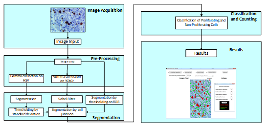Fig. 1.  Block diagram of the algorithm proposed.

variance [7][8], another factor that influences is the heterogenity of the stained sample [9]. Possible solutions to this issue have been proposed in previous research, but the main problems affecting cell detection in similar software remain: imperfection in collecting data such as noise, colour distortion and deformity in histopathological material at the stage of sample pigmentation, therefore a good calibration of the staining machine between IHC test should be made to avoid difference in pigmentation, this create a inter-laboratory variability on identical set of tumors [10].

In [11], for example, the results of the quantification algorithm were successful in analysing KI-67 with different image processing techniques such as thresholding, segmentation and labelling. However, the use of the ultra-erosion technique damaged valuable information for the evaluation of the sample.

In [12], they implement an algorithm based on mathematical description of cell morphology added with Support Vector Machine (SVM), obtaining great accordance between the digital image analysis and the “eyeballing” method.

On the other hand, M. Bouzid et al. show in [13] an interesting proposal with the use of special hardware: a multispectral camera with programmable light source. However, it increased the cost and availability of the solution. F. Kabir and N. Yusoff used in [14] the method of Random Forest (RF), consisting of predictive tree-like structures, each independent of the other, that obtain their data from different random vectors, but same distribution. RF has proved to perform better than other machine learning techniques, such as neural networks, support vector machines and k-nearest neighbors. The results of the tests, however, showed an accuracy of 72% in differentiating between malignant and benign tissue.

In this paper, an alternative solution is proposed on the basis of a digital image processing algorithm designed to quantify and provide more objective results regarding the level of cell proliferation based on marker KI-67. The algorithm involves statistical image processing techniques [15], adaptive thresholds [15][16], object segmentation and colour filtering [17]. Similarly,

it proposes an overlapping cell analysis and quantification method to improve the efficiency of cell detection. These techniques have been used together to obtain satisfactory results based on the problem. The results were indeed satisfactory, as presented at the end of this document.

In the following sections, the processing stages of the algorithm proposed in this paper will be described.

2. Description of the proposed algorithm

The proposed algorithm involves different processing parts and stages, as shown in Fig. 1. The scheme proposed contains the stages of image acquisition, pre-processing, segmentation, classification and counting. These steps will be described below.

2.1.  Image acquisition

Before being digitalised, the biopsy sample goes through an IHC process, which mixes the laminated sample with chemicals and special antibodies to achieve proper homogenous staining.

Currently, the procedure is performed automatically using the Ventana BenchMark XT stainer in line with the producer’s manual. After staining, the sample is placed under an Olympus BX53 digital microscope with a 40x magnifying lens, 50 images were chosen to study, all were given by chief of the department of anatomy pathology of Hospital Edgardo Rebagliati Martins, all samples were chosen randomly. The images of the biopsy sample (pre-treated by IHC) are obtained from a digital camera and an optical microscope. In this case, camera resolution was M0=2748 rows by N0=3584 columns with 40x zoom. The colour format of the original image (Fig. 2a) is RGB (Red, Green and Blue) called with 12 bits per primary colour component (36 bits/pixel). The primary components can be expressed as  and  .

All the parameters used in this paper were chosen taking in account the procedure mentioned previously to convert the biopsy sample into a digital image.

2.1.1.    Choosing the area of interest

The image can be cropped to select an area of interest. This procedure grants the pathologist the freedom to choose the area to analyse according to their own criteria and preference.

The selected area will have a resolution of M rows by N columns (this values may vary depending on the area selected by the specialist). The format is also RGB with primary components  and .

Figs. 2a and 2b show the original image and the cropped image, respectively.

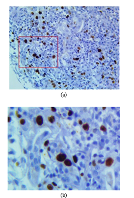Fig. 2.  (a) Original RGB image where the red square is the area to be zoomed. (b) Zoomed cropped image.

2.2.  Pre-Processing

Pre-processing aims to improve the quality of the image obtained in order increase the efficiency of segmentation algorithms. This process involves the following image processing blocks: Gamma correction on HSV (Hue, Saturation and Value) and Gamma correction on YCbCr (Luminance, Chrominance Blue, Chrominance Red).

2.2.1 Gamma correction on HSV

The cropped image expressed in its primary components  is converted to the HSV component  [15].

Gamma correction is applied with logarithmical effect to this component so as to enhance the contrast between the background (epithelium) and the proliferating cells. This will further increase the efficiency of segmentation algorithms. The conversion applied can be expressed as [17]:

Where  function generates the maximum value among  and .

The Gamma correction applied to can be expressed as [13]:

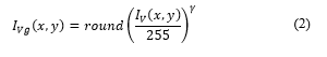where γ = 0.9 and round(x) return the approximate value to the nearest integer.

Fig. 3a shows image in RGB format; Fig. 3b shows   after applying (1) to ; and Fig. 3c shows , where non-proliferating or blue cells obtain a colour scheme similar to that of the background, making proliferating cells stand out. Likewise, in Fig. 3c, partially proliferating cells become evident.

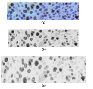Fig. 3. Image , (b)  and (c)

2.2.2. Gamma correction on YCbCr

In parallel with the process above, the cropped image expressed in its primary components  and is converted to the YCbCr component  the conversion can be expressed as [15]:

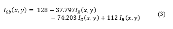Gamma correction is applied to this component with γ = 4 (exponential effect). This allows to displace Cb colour schemes from non-proliferating cells. Displacement from the original Cb dimensional space, shown in Fig. 4a. is shown in Fig. 4b. The image resulting from the process is expressed as , as shown in Fig. 5.

The correction applied allows to separate colour schemes and improve future segmentation of the two types of cells.

2.3.  Segmentation

In this process, objects corresponding to proliferating and non-proliferating cells are segmented. Segmentation is made from the corrected images and  obtained from the original image (Fig. 6).

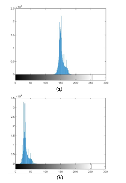Fig. 4.  (a) Original Cb (histogram) dimensional space. (b) Displaced Cb2 (histogram) dimensional space.

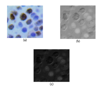Fig. 5. (a) Original image RGB. (b) Image  (c) Image  after application of Gamma correction.

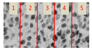Fig. 6. Image to be subjected to the proliferating cell segmentation process

2.3.1. Segmentation of proliferating cells

To separate the background (cell tissue of no interest for diagnosis) from the proliferating cells, it was decided to use local adaptive thresholds, which result from the probability density function (obtained by histogram) and first order statistical measures (mean and variance). The steps to achieve this process are as follows:

Step 1:

Image  is segmented in  segments. Image segments will have a spatial resolution of  rows by  columns. The segments of image  can be expressed as:

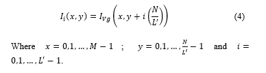Where ;  and .

In this case, we have  , because a more even segment is obtained in terms of noise and illumination (Fig.6.).

Step 2:

The histogram of each  segment is determined, which is defined as . In this case  represents each colour scheme from 0 to 255 (Fig. 7).

Step 3:

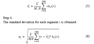
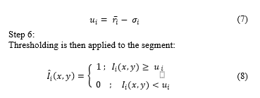
The mean value of each segment  is obtained:

Step 5:

The threshold to be used locally for each segment in order to separate cell tissue from the proliferating cell area is the result of the subtraction of the mean and standard deviation:

Step 7:

Finally, each segment thresholded  is placed in the original order so as to reconstruct an image with spatial resolution of  rows and  columns, which will be called and will contain the proliferating cell area as shown in Fig. 8.

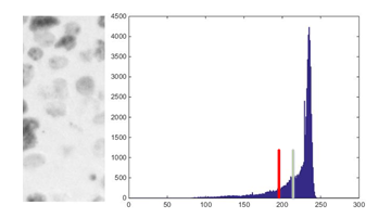Fig. 7. Example: Segment 1 of  ) and its histogram (in this case, the green bar indicates the mean value of the histogram and the red bar the threshold obtained).

2.3.2. Segmentation by Sobel filter and morphology

After identifying proliferating cells, it is necessary to spot non-proliferating cells in order to find the percentage of cells with proliferative activity in the image under evaluation .

For this process, image   obtained in the step above is used. The procedure is detailed below:

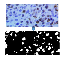Fig. 8. Original Image and resulting binary image  after the proliferating cell segmentation process.

Step 1:

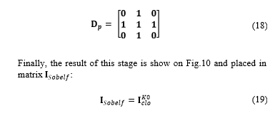
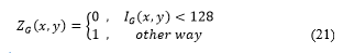
A thresholding filter is applied to    in order to segment non-proliferating cells. Thresholding can be expressed as:

The threshold was obtained from the study and evaluation of image histograms corresponding to various samples obtained. The result of the process is shown in Fig. 9.

Step 2:

Then, the Sobel filter [17] for edge detection is applied to binary images.

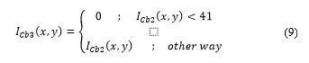
In this process, is convolved with each of the Sobel masks (horizontal and vertical) which are defined in matrix as [14]:

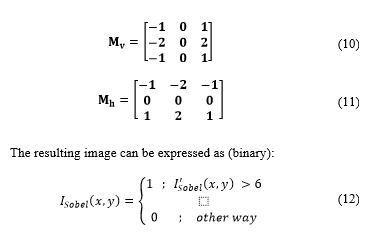
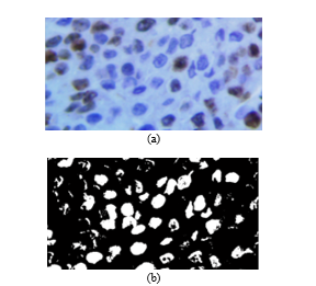Fig. 9.  (a) Original image. (b) Resulting image

Where: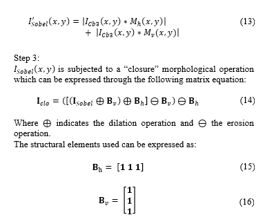

 is subjected to a “closure” morphological operation which can be expressed through the following matrix equation:

In order to reform the cells detected and not to distort the visual result, gap-filling is applied to the matrix cells . This operation can be expressed as [16]:

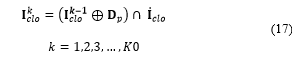Where  indicates the number of filling iteration,  denotes the intersection operation, and expresses the complement of matrix . Filling is made through  iterations until condition  is satisfied. The structuring element can be expressed as:

2.3.3. Segmentation by thresholding on primary components

At this stage, thresholding is applied to the primary RGB components to separate proliferating and non-proliferating cells from the epithelium (background). The thresholds used were obtained from experimental tests performed with images from different tissue samples. The procedure helps remove the area of the epithelium and highlight cells of interest. The steps of the procedure are as follows:

Step 1:

The primary components of the original image I are thresholded (Fig 11a):

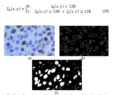Fig. 10. (a) Cropped original image. (b)Resulting Image after applying Sobel Filter. (c)Final Image  after gap-filling.

 2.3.4. Segmentation by cell junction

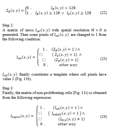
The combination of the proliferating and non-proliferating cell areas results in a binary image containing two types of segmented cells. This image is obtained as follows:

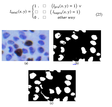Fig. 11. (a) Cropped original image. (b) Image    (c) Image .

However, one of the problems still present when the cells detected are counted is that some objects are made up of two or more joint or overlapped cells, which results in the algorithm giving a wrong diagnosis. In that sense, as in an acquisition with 40x magnification the average size of a cell is between 200 and 1500 pixels, we can consider that an object of  with a size above 1500 pixels is composed of more than one cell. This will definitely affect the counting, as an object is in principle composed of a single cell. To solve the problem, the following cell separation algorithm is proposed in order to minimise the counting error:

Step 1:

Consider a binary segment of  that contains object  with more than 1500 pixels. In this case,  …, and ; i.e. the segment size is    pixels.

Step 2:

We perform image rotation for different angles  ( ,  and . In this case, the rotation axis passes through the centre of image . The range of 15° between rotation angles was chosen based on the best results obtained in various tests of cell separation. Each turn generates an image that can be expressed as ,where  indicates the rotation angle. The spatial dimensions of each  is expressed as  rows by columns.

Step 3:

The horizontal projection  is obtained:

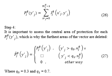Where  = 0.3 and  = 0.7.

Step 5:

Value is obtained, which is defined as the minimum value of the projection . In this case,  is the position where  is the minimum value.

Step 6:

The vector is then obtained:

Step 7:

The minimum value of vector  is obtained, which is defined as , where  is the angle corresponding to the minimum value of .

Step 8:

Then  is obtained from  :

Step 9:

Rotation of  over  is applied to restore the original orientation (although distortion is present due to the interpolation applied to the rotation process). After rotation, image  is obtained.

Step 10:

Finally, the block of image  is inserted in  (in the region where  was extracted).

Where  and   are the coordinates of the first pixel segment extracted .

Fig. 12a shows original areas of  containing objects made up of more than one cell. Fig. 12b shows the results obtained after applying the algorithm of cell separation.

2.4. Classification and counting of proliferating and non- proliferating cells

From the total number of cells detected in image , we proceed to classify and count proliferating and non-proliferating cells.

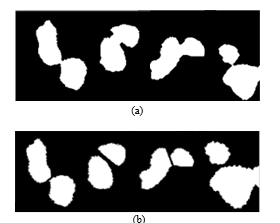Fig. 12.  (a) Samples with junction. (b) Samples after the separation process.

Cooperation with pathologists was managed so that the parameters of cell classification were correct and a good diagnosis could be achieved. In this case, doctors requested to classify proliferating cells into three sub groups: strongly proliferating, moderately proliferating and poorly proliferating. The classification criterion is based on the size of the cell area affected by the KI-67 protein.

Image is subjected to a labelling algorithm [16] that will label each cell detected as a   object. In this case,   is the object counter detected in the image. For a total of Q objects, we have k = 0,1,2, … Q-1.

2.4.1. Classification of Proliferating and Non-Proliferating Cells

For the classification stage, counters  (proliferating cell counter) and counter   (non-proliferating cell counter) are initialised.

is defined as the total number of objects or cells contained in . In this context,  is taken to be the object or cell number to be processed. In this case . We make  and carry out the following procedure:

Step 1:

A segment  of image is extracted consisting of rows and  columns, where   and . In this case,  is the image segment containing the object  detected in .

Step 2:

A flag  is updated through the following expression:

Where   and   are the coordinates of the first pixel of  in .

Step 3:

If the cell under evaluation is considered proliferating and the counter   increases by one unit. Otherwise, the counter  increases. Within the requirements of doctors, a sub classification of proliferating cells was made in 3 levels of proliferation: strongly proliferating, moderately proliferating and poorly proliferating.

In this way, when  , steps 4 to 9 are executed.

Step 4:

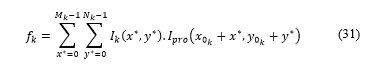
A temporary matrix  consisting of  rows and  columns is generated and applied: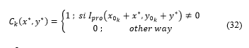

Step 5:

We count each pixel belonging to an area that reacted to KI-67:

Step 9:

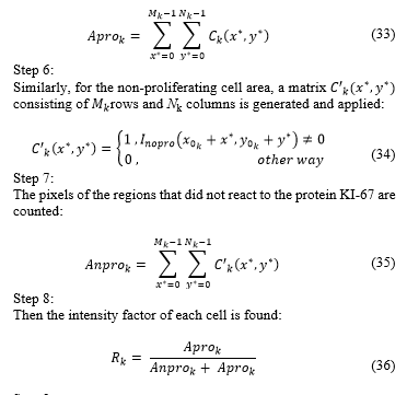
Flags of proliferation   ,  and are updated:

For each  where there is only one active flag ( ).

Three counters (initialised to zero), defined as strong, medium and weak, are updated. They are updated as   follows:  if , the strong counter is incremented by one; if , the medium counter is increased by one; if , the weak counter is increased by one. These counters store the amount of subclassified cells. Note that strong + medium + weak = . This data is granted to the pathologist for evaluation and diagnosis, as shown in Table 1.

Then,  increases by one unit and we go back to step 1. The procedure ends when .

Step 10:

After evaluating all the cells, we find the percentage of proliferating cells and obtain:

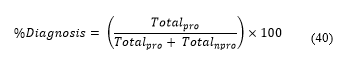 Table 1. Results after test.

Total counted nucleus	Quantity	Percentage (%)
Negative nucleus	94	88
Positive nucleus	13	12
Total	107	100
Positive counted nucleus
Strong positive nucleus	2	15
Medium positive nucleus	7	54
Weak Positive Nucleus	4	31

3. Results

To prove that the software can be used by specialists, the results obtained by it had to be validated against the results provided by doctors; they were requested to make the same analysis on equal samples. The doctors that carried out the tests are specialised in pathology and work in different institutions in the city of Lima.

Table 2, 3, 4, 5 and 6 show the results obtained in different cases. When comparing the results obtained by the application against the diagnosis given by doctors, it was concluded that, in samples with a clear KI-67-active cell rate (either in a very small or very high percentage in proportion to the total number of cells), doctors using the eyeballing technique obtain results very similar to those of the application. But when samples present some difficulty at the time of counting, it is observed that the results among doctors are poorly correlated with each other and only a few can give a diagnosis similar to that of the application. This is because doctors are subject to different stimuli that influence their performance and they have different counting methods, such as hotspots, random areas, or groups near adjacent hotspots [7], while the software will always proceed in the same way.

In Figure 13 it is shown a section of an evaluated image by both the medical specialist and the developed algorithm. Five cells have been enumerated and marked in a rectangle, named: cell 1, cell 2, cell 3, cell 4 and cell 5.

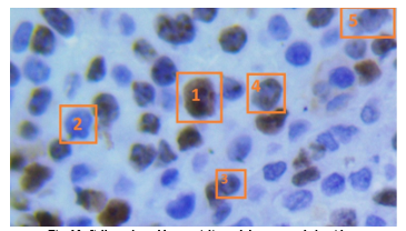Fig. 13. Cells evaluated by specialist and the proposed algorithm.

For cell 1, both medical specialist and proposed algorithm confirmed that represent a proliferative cell, meaning it was stained in brown color by the IHC process.

For cell 2, again both specialist and algorithm concurred that the cell was non-proliferative, stained with a blue tone by the IHC process. In case of cell 3 and 5, the staining was lower than cell 1, specialist marked the cell as non-proliferative and the algorithm marked as proliferative, is in this scenario in which the subjectivity of human eye turn the proliferation index and can occur divergence in the diagnosis. In case of cell 4, shows partial staining and both specialist and algorithm matched as proliferative.

To demonstrate the error trend, the table below shows the calculus of coincidence between the software and the specialists, and its measuring using the Kappa coefficient.

Defining Kappa coefficient as [18]: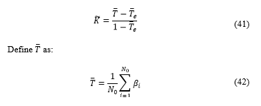

Where  is the total number of category, in this case two categories  : Luminal A, and Luminal B, as explained on [6], Luminal A if diagnosis was <20% and Luminal B if was ≥20%.

 is defined as: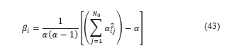

Where  is the number of occurrences from a category,  is the number of times the specialist chose a diagnosis in the category  and the software chose category .

Finally:

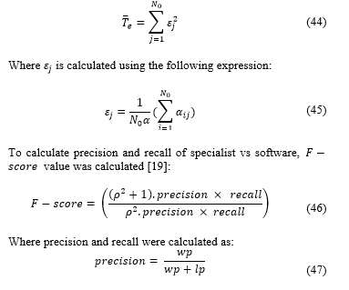Where  is calculated using the following expression:

And:

Where:

: true positive, a cell that specialist said was proliferative and algorithm said was proliferative.

: false positive, a cell that specialist said wasn’t proliferative and algorithm said it was proliferative.

: false negative, a cell that said specialist said was proliferative but algorithm said wasn’t proliferative.

 is considered balanced so:

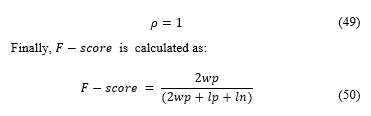
The average result for F-score of the samples was of 0.8764, showing a high concordance between the software and specialist. The software detects a greater number of cells than the specialist, so the F-score is not perfect, however, these cells not accounted were mostly discarded by specialist errors.

As shown in the Tables 2, 3, 4, 5 and 6 there is a remarkable variation among specialists in the Luminal B diagnosis made by counting. The poor agreement in the diagnosis is due to the difference between stained and non-stained nuclei as rapidly observed by the specialist. Nevertheless, two specialists gave the same result as the software; it should be noted that a proliferation index >20% is needed to share the same diagnosis.

Tables 7, 8 and 9 show the difference among specialists when giving their diagnosis. The Kappa index among specialists is not constant, an average of 0.6863, which demonstrates, once again, the difference generated by the subjective analysis by eyeballing [9][10].

Table 2. Comparison Software vs. Specialist 1

Specialist 1: Kappa
Specialist 1   Software	Luminal A	Luminal B	TOTAL
Luminal A	7	3	10
Luminal B	0	9	9
TOTAL	7	12	19

Table 3. Comparison Software vs. Specialist 2

Specialist 2: Kappa
Specialist 2   Software	Luminal A	Luminal B	TOTAL
Luminal A	7	3	10
Luminal B	0	9	9
TOTAL	7	12	19

Table 4. Comparison Software vs. Specialist 3

Specialist 3: Kappa
Specialist 3   Software	Luminal A	Luminal B	TOTAL
Luminal A	10	0	10
Luminal B	0	9	9
TOTAL	0	9	19

Table 5. Comparison Software vs. Specialist 4

Specialist 4: Kappa
Specialist 4   Software	Luminal A	Luminal B	TOTAL
Luminal A	10	0	10
Luminal B	0	9	9
TOTAL	0	9	19

Table 6. Comparison Software vs. Specialist 5

Specialist 5: Kappa
Specialist 5   Software	Luminal A	Luminal B	TOTAL
Luminal A	10	0	10
Luminal B	2	7	9
TOTAL	12	7	19

Table 7. Comparison Specialist 1 vs. Specialist 2

Specialist 1 vs Specialist 2: Kappa
Specialist 1   Specialist 2	Luminal A	Luminal B	TOTAL
Luminal A	6	1	7
Luminal B	1	11	12
TOTAL	7	12	19

Table 8. Comparison Specialist 2 vs. Specialist 4

Specialist 2 vs Specialist 4: Kappa
Specialist 2   Specialist 4	Luminal A	Luminal B	TOTAL
Luminal A	7	0	7
Luminal B	4	8	12
TOTAL	11	8	19

Table 9. Comparison Specialist 1 vs. Specialist 5

Specialist 1 vs Specialist 5: Kappa
Specialist 1   Specialist 5	Luminal A	Luminal B	TOTAL
Luminal A	7	3	10
Luminal B	0	9	9
TOTAL	7	12	19

4. Conclusions

In this publication, an algorithm to quantify the proliferative index of the KI-67 marker in histological samples of breast tissue has been developed that proves to give results more reliable than results given by specialist, thanks to image processing techniques, this algorithm can help to provide a better diagnostic to treat breast cancer when applied the result with other biomarkers to diagnose cancer.

A software application was developed. It meets the standards and criteria that pathologists use for the evaluation of the immunohistochemistry method and it is approved by specialists, as they consider that, when testing the software in their work centres, results are reliable.

The iterative algorithm of cell separation is computationally heavy and must be optimised for the comfort of physicians.

In developing the software, in cooperation with medical advisors, new limitations and standards emerged; this is the only way to consolidate a multidisciplinary project.

The quality of the images provided must have some standard sharpness and correct pigmentation to be processed by the application.

Conflict of Interest

The authors declare no conflict of interest.

1.  E. Poquioma. “Situación del cáncer de mama en el Perú”. Presentation. Instituto Nacional de Enfermedades Neoplásicas (INEN), 2008.
2.  C. Ramos, D. Venegas. “Análisis de la Situación del Cáncer en el Perú”. Presentation. Dirección General de Epidemiología, Ministerio de Salud del Perú, 2013.
3.  S. Coronato, G. Laguens, O. Spinelli, W. Di Girolamo. “Marcadores tumorales en cancer de mama” MEDICINA (Buenos Aires), 63, 73-82, 2002.
4. B. Hirata, B. Karina, et al. “Molecular markers for breast cancer: prediction on tumor behavior.” Disease markers, 2014. http://dx.doi.org/10.1155/2014/513158
5.  H. Xin et al. “Ki-67 is a valuable prognostic predictor of lymphoma but its utility varies in lymphoma subtypes: evidence from a systematic meta-analysis.” BMC cancer, 14, 153, 2014. http://doi:10.1186/1471-2407-14-153
6. S. Bustreo, S. Osella-Abate, et al. “Optimal Ki67 cut-off for luminal breast cancer prognostic evaluation: a large case series study with a long-term follow-up” Breast Cancer Res Treat, 157(2), 363–371, 2016. 10.1007/s10549-016-3817-9
7.  L. Fulawka, A. Halon. “Ki-67 evaluation in breast cancer: The daily diagnostic practice” Indian J. Pathol Microbiol, 60(2), 177-184, 2017. http://doi:10.4103/IJPM.IJPM_732_15
8.  Gudlaugsson, E., Skaland, I., Janssen, E. A., Smaaland, R., Shao, Z., Malpica, A., … & Baak, J. P. (2012). Comparison of the effect of different techniques for measurement of Ki67 proliferation on reproducibility and prognosis prediction accuracy in breast cancer. Histopathology, 61(6), 1134-1144.
9.  Zhong, F., Bi, R., Yu, B., Yang, F., Yang, W., & Shui, R. (2016). A comparison of visual assessment and automated digital image analysis of Ki67 labeling index in breast cancer. PloS one, 11(2), e0150505.
10.  Koopman, T., Buikema, H. J., Hollema, H., de Bock, G. H., & van der Vegt, B. (2018). Digital image analysis of Ki67 proliferation index in breast cancer using virtual dual staining on whole tissue sections: clinical validation and inter-platform agreement. Breast cancer research and treatment, 169(1), 33-42.
11.  V. Anari, P. Mahzouni, R. Amirfattahi “Computer-aided Detection of Proliferative Cells and Mitosis Index in Inmunohistichemically Images of Meningioma” In 6th Iranian Conference on Machine Vision and Image Processing, Isfahan, Iran. IEEE, 2010. 10.1109/IranianMVIP.2010.5941151
12.  Grala, B., Markiewicz, T., Kozłowski, W., Osowski, S., Słodkowska, J., & Papierz, W. (2009). New automated image analysis method for the assessment of Ki-67 labeling index in meningiomas. Folia Histochemica et Cytobiologica, 47(4), 587-592.
13.  M. Bouzid, A. Khalfallah, A. Bouchot, M. Selim, F. Marzani. “Automatic Cell Nuclei Detection: a Protocol to Acquire Multispectral Images and to compare results between colour and multispectral images” in SPIE Photonics West, BIOS, Imaging, Manipulation and Analysis of Biomolecules, Celles and Tissues XI, San Francisco, United States, 2013. doi.10.1117/12.2001980
14.  K. Ahmad, N. Yusoff. “Breast Cancer Types Based on Fine Needle Aspiration Biopsy –Data Using Random Forest Classifier” in I 13th International Conference on Intellient Systems Design and Applications, Bangi, Malaysia. IEEE, 2013. doi.10.1109/ISDA.2013.6920720
15.  R. Gonzalez, R. Woods. Digital Image Processing, 3rd. Ed., Prentice Hall, 2008.
16.  T. Chun-Ming, L. His-Jian. “Binarization of Colour Document Images via Luminance and Saturation Colour Features” IEEE Transactions on Image Processing, 11(4), 2002. 10.1109/TIP.2002.999677
17. R. Gonzales, R. Woods, E. Eddins. Digital Imaging Processing Using Matlab, 2nd Ed., Mcgraw Hill, 2010.
18. J.L Fleiss. “Measuring Nominal Scale Agreement Among Many Raters” Psycological Bulletin, 76(5): 378-382, 1971. http://dx.doi.org/10.1037/h0031619
19.  M. Sokolova, N. Japkowicz, S. Szpakowicz. “Beyond Accuracy, F-Score and ROC: A Family of Discriminant Measures for Performance Evaluation” In AI 2006: Advances in Artificial Intelligence, Lecture Notes in Computer Science (vol. 4304), 2006. DOI: 10.1007/11941439_114

(Click Here)

(Click Here)