1. Introduction

Delay Tolerant Networks (DTNs) [1] are one of the most attractive progresses in Mobile Ad Hoc Networks (MANETs), which become dominant due to the emergence of the intelligent devices equipped with wireless communication facilities. Historically, DTN concepts were emerged in the interplanetary environment studies. After that, the DTN concepts grew to cover other types of networks. As examples of DTN networks we cite: disaster environments [2], under water communications [3], rural remote patient monitoring [4], animal habitat monitoring and network sensors for wildlife tracking [5], vehicular delay tolerant networks (VDTN) [6], surveillance for regions on the earth surface [7] and any network with frequent links disruptions due to environmental features changing. It should be noted that the routing in DTN is more difficult than in MANET. This is due to the lack of information about network topology in DTN networks. DTN Networks are characterized as intermittent connectivity with often end-to-end path interruption and topology alterations. Once a connection is established, there is no guarantee to maintain it until the end of the communication. This is caused by the mobility of the nodes, which can lead to instability of the paths between sources and destinations. To overcome this inherent problem, DTN networks rely on Store-Carry-Forward transport paradigm. In this paradigm, when a source node wants to transmit a message to a destination node, it sends the message to the neighboring nodes, referred to as relay nodes or candidate nodes. The relay nodes do the same until the message delivered finally to its destination. This paradigm is called opportunistic transport and the network on which is based is called opportunistic network. Despite opportunistic contacts, sporadic connectivity and limited resources, opportunistic networks attempt to facilitate the exchange of information between users (nodes). To this end, all internet and mobile Ad-hoc networks routing protocols need to be redesigned according to this paradigm. For more than two decades researchers have developed many routing protocols for opportunistic networks. Some of these protocols are simple and rely solely on flooding the network with messages’ copies in the hope that the messages will reach their destination. Intricate protocols try to forward copies of messages only to the nodes that are best placed to deliver messages to their destination at the lowest cost. In the literature, there are many classifications of routing protocols in opportunistic networks. Some of them are flooding-based and quota-based routing protocols [8]. In the flooding-based routing protocols, each node floods the network with messages’ copies in the hope that one of them will reach its destination. In [9], Epidemic was presented as example of flooding-based  routing protocols. Flooding-based routing protocols work very well if the network has unlimited buffer sizes and all nodes are rechargeable. However, in opportunistic networks with limited resources, flooding-based protocols are poor. To control flooding in these protocols, a lot of protocols have been proposed. These protocols are termed as guided-based routing protocols [10] and are considered as a subcategory of the flooding-based routing protocols. Guided-based routing protocols forward messages only to the nodes that are most likely to reach the destination. This is done by allowing the forwarding decision of the message to be based on a utility metric calculated according to certain criteria. Some of these criteria depend on the contact rate, as in PRoPHET protocol [11]. Some other utility metrics are calculated based on the  path cost to the destination, as in the MaxProp routing protocol [12].

In the quota-based routing protocols, the router imposes an upper limit on the number of messages’ copies in the network. For instance, we cite Spray and Wait (SaW) [13], Spray and Focus (SaF) [14] and Encounter Based routing (EBR) [8].

In this paper, we performed an analytical study on the performance of the most common routing protocols in opportunistic networks. These protocols are: Epidemic, PRoPHET, MaxProp, Spray and Wait, Spray and Focus and EBR. These protocols are selected precisely because of their outstanding performance and because they are often used as benchmarks in most studies. The experiments were conducted in resource-poor environments, non-rechargeable nodes, and limited memory. In such harsh environments, it is difficult to make a precise statement about what kind of services can be provided [15]. Therefore, our study serves to make comparisons and conclusions that help designers to improve performance in such challenging networks. To our knowledge, our work is one of the rare studies that could provide an in-depth analysis of the behavior of the most common routing protocols of resource-constrained opportunistic networks. The study also includes key recommendations for designing a high-performance routing protocol.

The remainder of this work is organized as follows: in section 2 the related works are presented. Opportunistic routing protocols explanations are presented in section 3. Section 4 introduces the used system model. Performance evaluation and the settings of the simulation are presented in section 5. In section 6, the results are presented followed by discussions. Design guidelines are presented in section 7. Finally, section 8 provides the conclusion of this work.

2. Related Works

Routing mechanisms in opportunistic networks are one of the most important elements that play a major role in their performance. Therefore, investigating the effectiveness of routing protocols in opportunistic networks is an important topic. Moreover, the store-carry-forward transport paradigm makes the routing performance analysis more complex and challenging than other networks. In view of the importance of the subject, we find in the literature a lot of researches that have addressed this topic.

Authors in [16] compared the performance of several routing protocols in opportunistic networks. The experiments were performed with different numbers of nodes at different speeds. However, this research did not take into account traffic loads, message lifetime, buffer size and energy consumption. Despite the valuable results of this research, it does not focus on opportunistic networks with limited resources.

Several representative routing protocols in opportunistic networks were investigated in [17]. The simulations performed with different numbers of nodes and traffic loads. The simulation time was 24 hours in all experiments and all nodes were rechargeable. However, this research did not highlight resource constraints in opportunistic networks.

In [18], authors perform a performance analysis research of eight routing protocols of delay tolerant networks. The eight protocols were compared in different traffic loads and message lifetimes. All nodes were rechargeable and equipped with buffers of 50 MB. in all experiments, simulation time was 6 hours. However, this study did not address the resource consumption issues which is a major concern in the limited resource opportunistic networks.

Authors in [19] highlight the energy consumption issue in opportunistic networks. they compared the performance of five of the most common routing protocols. The five protocols were compared in different numbers of nodes and hop counts. However, the study did not address the buffers consumption issue which is one of the most important resources in opportunistic networks.

Complexity and scalability was the main objective of comparison in [20]. The authors compared three routing protocols: Epidemic, PRoPHET and First Contact. Despite the valuable results, they did not take into account the consumption of network resources.

Authors in [10] compared the performance of four well-known routing protocols in opportunistic networks. the comparison was carried out by changing the values of message lifetime, buffers, traffic load and the number of nodes. In addition to the results of the comparisons, the authors addressed a set of guidelines to improve routing protocols. In spite of the beneficial results, the research did not include the effect of energy consumption on the performance of the routing protocol.

Our research differs from previous studies in that it mainly highlights the issue of the limited resources of opportunistic networks. Our study did not overlook the limitations of energy and memory in all analyzes. We firstly described the most common protocols and presented their algorithms. Thereafter, we carried out a comparative study of these protocols using exhaustive performance testing experiments with different numbers of nodes, traffic loads, message lifetime, and buffer size.

3. Opportunistic Routing Protocols

3.1. Epidemic Routing Protocol

The authors in [9] propose the Epidemic routing protocol, which is classified as a flooding-based routing protocol. It is historically the first protocol in opportunistic networks. It works as follows: When a node encounters another node, it gives it a copy of the messages it has and is not in possession of the other node. In fact, both nodes exchange the so-called summary vector, which contains their respective message IDs. The messages remain in buffers until they are delivered to their destination or dropped due to their expired lifetime. The pseudocode of the Epidemic router is shown in Algorithm 1.

If all nodes in the network are rechargeable and have unlimited buffer sizes, the EPIDEMIC routing protocol theoretically achieves the highest transfer rate and lowest latency. However, in opportunistic networks with limited resources, EPIDEMIC is the neediest protocol for network resources in terms of energy and buffer consumption.

ALGORITHM 1.  EPIDEMIC ROUTING PROTOCOL
1:	Let nx and ny two nodes in an opportunistic network.
2:	Let DropExpireMessages(nx) a procedure for dropping expired messages in node nx  .
3:	Let ExchangeSummaryVectors(nx, ny) a procedure for exchanging the summary vectors of both nodes.
4:	if nx meets ny then
5:	DropExpireMessages(nx).
6:	ExchangeSummaryVectors(nx, ny).
7:	for each message mx  in node nx do
8:	if mx did not exist in ny then
9:	Forward a copy of mx to  ny
10:	end if
11:	end for
12:	end if

3.2. PRoPHET Routing Protocol

PRoPHET stands for a Probabilistic Routing Protocol using History of Encounters and Transitivity [11]. In PRoPHET, messages are routed  based on the  destination’s encounter probability which is termed as delivery predictability, and denoted by P_(a,b) ∈ [0, 1], where a is a node among nodes in the network and b is the destination node. Actually, the delivery predictability metric is computed according to three equations depending on the happened event. If the node   meets another node , the delivery predictability metric is updated according to equation (1).

P_(a,b) = P_{(a,b)old +} (1 –  P_(a,b)old) × P_(a,b)init                               (1)

where P_(a,b)old is the previous delivery predictability value and P_(a,b)init is the starting value.

The longer the interval between the two meetings between any two nodes, the less likely they will see each other in the future. Hence, the delivery predictability is aged (reduced) based on equation (2).

P_(a,b) = P_(a,b)old ×                                                          (2)

where  is the aging constant and k is the number of time units that have elapsed since the last measurement was reduced.

Also, a transitive property is formed based on the observation that shows if a node  frequently meets a node  and node  frequently meets a third node , then there is a high probability that node c will be a good choice for forwarding messages to node a. The delivery predictability  is updated according to this transitive property as follows:

P_(a,c) = P_{(a,c)old +} (1- P_(a,c)old × P_(a,b) × P_(b,c) × β)                              (3)

where β is a constant that decides how large the effect of the transitivity should have on the delivery predictability.

Now, the routing strategy that is followed is simple. When a node encounters another node, the messages will be forwarded (copied) to the other node only if the delivery predictability value for the message’ destination of the encountered node is higher. The pseudocode for the PRoPHET routing protocol is presented in Algorithm 2.

ALGORITHM 2.  PROPHET ROUTING PROTOCOL
1:	Let nx and ny two nodes in an opportunistic network.
2:	Let DropExpireMessages(nx) a procedure for dropping expired messages in node nx  .
3:	Let ExchangeSummaryVectors(nx, ny) a procedure for exchanging the summary vectors of both nodes.
4:	Let UpdateDeliveryPredictability() a procedure for recalculating the delivery predictability values for all known destinations.
5:	Let nD the destination node of the message m.
6:	Let P(n, nD) the value of the delivery predictability of n to deliver the message to its destination nD.
7:	if nx meets ny  then
8:	DropExpireMessages(nx)
9:	ExchangeSummaryVectors(nx, ny)
10:	UpdateDeliveryPredictability()
11:	for each message mx in node nx do
12:	if mx did not exist in ny then
13:	if P(ny, nD) > P(nx, nD) then
14:	Forward a copy of mx to ny
15:	end if
16:	end if
17:	end for
18:	end if

PRoPHET is considered a guided-based routing protocol. This is because messages are routed to their destinations using the Delivery Predictability Metric. However, it still suffering from high overhead and high consumption of network resources.

3.3. MaxProp Routing Protocol

MaxProp [12] is motivated by the limitations of some existing systems, as they focus on short-range targets and can not remove obsolete messages from the network. Therefore, MaxProp removes outdated messages from the network buffers and prevents the double data spread on the same node. Each node in the network maintains a vector list which contains the estimation of encountering of all other nodes in the network. So, for any two nodes, denoted a and  b , in a network of S nodes, the initial probability to meet each other is given by equation (4).

P_(a,b) =1/(S-1)                                                                               (4)

If the node a meets the node b, the probability is updated by increasing P_(a,b) with 1, and then all other probabilities of meeting between the node a and the other nodes in the network are normalized.

ALGORITHM 3.  MAXPROP ROUTING PROTOCOL
1:	Let nx and ny two nodes in an opportunistic network.
2:	Let DropExpireMessages(nx) a procedure for dropping expired messages in node nx  .
3:	Let ExchangeSummaryVectors(nx, ny) a procedure for exchanging the summary vectors of both nodes.
4:	Let UpdateDeliveryPredictabilities() a procedure for recalculating the delivery predictability values.
5:	Let CostCalculation(nD) a procedure to calculate the cost of the destination of the message mx.
6:	Let ExchangeAcknowledgments() a procedure to exchange the acknowledgments lists of the delivered messages.
7:	if nx meets ny  then
8:	DropExpireMessages(nx)
9:	ExchangeSummaryVectors(nx, ny)
10:	UpdateDeliveryPredictabilities()
11:	ExchangeAcknowledgments()
12:	Delete acknowledged messages
13:	for each message mx in node nx do
14:	if (the message’ hop counts < threshold) then
15:	if  the message has the lowest hop count then
16:	Forward a copy of mx to ny
17:	end if
18:	end if
19:	CostCalculation(nD)
20:	if (A room is needed for an incoming message) then
21:	if  (mx has the biggest  cost) then
22:	Delete mx
23:	end if
24:	end if
25:	end for
26:	end if

Based on these probabilities, MaxProp computes destinations costs. Consequently, a message scheduling is done in each node based on these costs which will be used later for making the forwarding and dropping decisions. The pseudo code of MaxProp  is given by Algorithm 3.

Although MaxProp can choose the optimal delivery path, the method of estimating delivery costs used in this work is fast and not considered accurate [21]. However, in terms of overhead and resource consumption, MaxProp is better than PRoPHET [10].

3.4. Spray and Wait Routing Protocol

Spray and Wait (SaW) routing protocol is proposed in [13] to set an upper bound on the number of messages in the network. It is categorized as a quota-based routing protocol. The idea in SaW protocol is to associate a number L for each created message. This number defines the maximum number of copies that is allowed for the message in the network. the binary version of SaW protocol works as follows: When two nodes come together and exchange messages in their possession, the number L of copies of each message is equally distributed. The equally split process continues until the number of copies reaches one, then the node keeps a single copy of the message until it is delivered to its destination or it is dropped due to expiration. Therefore, this protocol is divided into two phases: Spray phase and the Wait phase. In the Spray phase, the number of copies is distributed until it reaches to one. In the Wait phase, a node waits until it meets the destination of the message. Algorithm 4 shows the pseudo code of SaW routing protocol.

Although SaW performs better than flooding-based routing protocols in term of overhead and resources consumption, performance degradation may occur because of the blind selection of the candidate node to carry the message.

ALGORITHM 4.  BINARY SaW ROUTING PROTOCOL
1:	Let nx and ny two nodes in an opportunistic network.
2:	Let DropExpireMessages(nx) a procedure for dropping expired messages in node nx  .
3:	Let ExchangeSummaryVectors(nx, ny) a procedure for exchanging the summary vectors of both nodes.
4:	Let Lmx the initial number of the copies that are allowed for the message mx in the network.
5:	Let ExchangeAcknowledgments() a procedure to exchange the acknowledgments lists of the delivered messages.
6:	if nx meets ny  then
7:	DropExpireMessages(nx)
8:	ExchangeSummaryVectors(nx, ny)
9:	ExchangeAcknowledgments()
10:	Delete acknowledged messages
11:	for each message mx in node nx  do
12:	if (Lmx > 1) then
13:	Lmx  ← Lmx /2
14:	Forward mx to ny
15:	else if  (ny is the destination of  mx) then
16:	Forward mx to ny
17:	Add mx to the acknowledgment list
18:	end if
19:	end for
20:	end if

3.5. Spray and Focus Routing Protocol

Spray and Focus (SaF) is proposed in [14]. SaF is similar to the SaW protocol. In fact, it uses the same first Spray phase, but it uses the phase of focus instead of the wait phase. In the Wait phase, the node that has a single copy of the message waits until it reaches the destination, or the message is expired. However, in the focus phase, the message will be forwarded to other nodes if only a single copy of the message remains in the node in order to accelerate the process of reaching the destination. The message forwarding decisions in the focus phase are made based on a utility metric that is estimated based on the contact history information. The pseudocode of the SaF routing protocol is shown in Algorithm 5.

ALGORITHM 5.  SaF ROUTING PROTOCOL
1:	Let nx and ny two nodes in an opportunistic network.
2:	Let DropExpireMessages(nx) a procedure for dropping expired messages in node nx  .
3:	Let ExchangeSummaryVectors(nx, ny) a procedure for exchanging the summary vectors of both nodes.
4:	Let Lmx the initial number of the copies that are allowed for the message mx in the network.
5:	Let UpdateDeliveryPredictabilities() a procedure for recalculating the delivery predictability value.
6:	Let ExchangeAcknowledgments() a procedure to exchange the acknowledgments lists of the delivered messages.
7:	Let nD  the destination node of a message m.
8:	if nx meets ny  then
9:	DropExpireMessages(nx)
10:	ExchangeSummaryVectors(nx, ny)
11:	ExchangeAcknowledgments()
12:	Delete acknowledged messages
13:	UpdateDeliveryPredictabilities()
14:	for each message mx in node nx  do
15:	if  (ny is the destination of  mx) then
16:	Forward mx to ny
17:	Add mx to the acknowledgment list
18:	Continue (break for loop)
19:	end if
20:	if (Lmx > 1) then
21:	Lmx  ← Lmx /2
22:	Forward mx to ny
23:	else if ( P(ny, nD) > P(nx, nD) )  then
24:	Forward a copy of mx to ny
25:	end if
26:	end for
27:	end if

Although SaW and SaF succeed in limiting the resource consumption, they still depending on the blind selection of the next hop in the Spray phase. Therefore, several solutions have been proposed to improve them in order to avoid blind selection of the relay nodes. As an example, we cite [22].

3.6. EBR Routing Protocol

An Encounter-Based Routing protocol (EBR) is proposed in  [8]. Similar to SaW and SaF, EBR is considered a quota-based routing protocol because it limits the number of copies of the message in the network. Thus, the number of copies of a message m_x in the node n_x, is limited by a fixed threshold L. When a node  encounters a node , the number of copies of the message m_x is distributed between the two nodes according to their previous encounter rate denoted by EV. To get more accurate EV values, the EBR protocol uses the concept of the exponentially weighted moving average. If CW stands for the current window, which is the number of encounters within the current time interval, EV is periodically recalculated using equation (5).

EV = α × CW + (1- α) × EV                                                       (5)

where α is a weighting constant. The pseudocode of the EBR routing protocol is presented in Algorithm 6.

ALGORITHM 6.  EBR ROUTING PROTOCOL
1:	Let nx and ny two nodes in an opportunistic network.
2:	Let DropExpireMessages(nx) a procedure for dropping expired messages in node nx  .
3:	Let ExchangeSummaryVectors(nx, ny) a procedure for exchanging the summary vectors of both nodes.
4:	Let Lmx the initial number of the copies that are allowed for the message mx in the network.
5:	Let ExchangeAcknowledgments() a procedure to exchange the acknowledgments lists of the delivered messages.
6:	if  meets  then
7:	DropExpireMessages(nx)
8:	ExchangeSummaryVectors(nx, ny)
9:	ExchangeAcknowledgments()
10:	Delete acknowledged messages
11:	if  (CurrentTime > NextUpdateTime) then
12:	EVnx ← α × CW + (1- α) × EVnx
13:	CW ← 0
14:	NextUpdateTime ← CurrentTime+ NextUpdateTime
15:	end if
16:	for each message mx in node nx do
17:	if  (ny is the destination of  mx) then
18:	Forward mx to ny
19:	Add mx to the acknowledgment list
20:	Continue (break for loop)
21:	else
22:	Send [Lmx×EVny/( EVnx+ EVny)]  copies of mx to ny
23:	Lmx ← [1- Lmx×EVny/( EVnx+ EVny) ]
24:	end if
25:	end for
26:	end if

4. System Model

We consider an opportunistic network with the well-known Opportunistic Network Environment Simulator (ONE) [23]. ONE is a Java-based simulation program. It is designed primarily for opportunistic networks. Source codes are available in [24]. All experiments are conducted using real live mobility of the following patterns: pedestrians, bicycles, motorcycles, and drivers of faster and slower cars. All nodes use Bluetooth as the communication medium. Each node is equipped with a battery with a limited power budget of 800 mAh. The size of the generated messages is 128 KB. The size of the world is 4500 × 3400. No assignment to special routes or maps to a group. Downtown Helsinki (pedestrian streets and streets) is the environment of our experiments. We assume that all nodes employ the Shortest Path Map-Based motion model and all nodes are not rechargeable.

5. Performance Evaluation

Since we want to measure the performance of protocols in opportunistic networks with limited buffers and limited energy, the effectiveness of these routing protocols should be observed with different values of buffer sizes and their performance evaluated taking into account the continuous energy consumption over time.

5.1. Performance metrics

We consider four metrics to evaluate the performance of  the routing protocols. The performance metrics are explained as follows:

• Delivery Ratio: It is the ratio of the total number  of delivered messages D to the total number of created messages It is given by the equation (6).

• Overhead Ratio: It reflects how many redundant messages are relayed to deliver one message. It simply reflects transmission cost in a network. It is given by equation (7).

where F is the total number of forwarded messages by the relays nodes.

• Average Latency: It is the average of delay, i.e., the time between the creation of messages and their reception by the final destination. It is given by equation (8).

where t_Di is the time at which the i^th message was delivered, t_Ci is the time at which the i^th message was created and n is the number of delivered messaged.

• Average buffer occupancy: the percentage of memory fullness.

5.2. Simulation Settings

The network parameters used in all experiments are listed in Table 1.

6. Results and Discussion

Table 2 summarizes the obtained results from all experiments. The numbers listed in the table are the minimum and maximum values.

Table 1: Simulation settings.

Nodes	Pedestrian	Bicycles	Bikes	Drivers1	Drivers2
Speed range (m/sec)	0-1.5	4-10	16-32	33 – 65	65 – 120
Buffer sizes (MB)	2, 4, 6, 8, 10, 12, 14, 16
Simulation Time (Hours)	12, 48
Number of nodes	10,30,50,70,90
Message generation rate (Msgs/Hour)	7, 18, 33, 103, 600
TTL (Hours)	1, 3, 6, 9, 12
Initial energy budget (mAh)	800
Energy expenditure for scanning (j/hour)	0.1
Energy expenditure for transmitting/receiving (J/hour)	15
PRoPHET parameters	P(a,b)init = 0.75; β = 0.25; γ = 0.98
SaW parameters	L = 8
SaF parameters	L = 8
EBR parameters	α = 0.85; CW = 30; L = 8

Table 2: Summary of results.

Impact of		Simulation Time & Buffer size	Number of Nodes & Buffer size	Traffic Load & Buffer size	TTL & Buffer size
Parameters		TTL=300 minutes TL=288 Messages/hour N=50 nodes BS = 2;4;6;8;10;12;14;16 MB ST = 6;12;18;24;30;36;42;48 Hours	TTL=300 minutes TL=288 Messages /hour ST=12Hours BS = 2;4;6;8;10 MB N=10;30;50;70;90 nodes	TTL=300 minutes ST=12Hours N=50 nodes BS = 2;4;6;8;10 MB TL = 7;18;33;103;600 Message/hour	ST=12Hours TL=288 Messages /hour N=50 nodes BS = 2;4;6;8;10 MB TTL =1;3;6;9;12 Hours
Delivery ratio	Epidemic	0.0271 – 0.2496	0.0536 – 0.46	0.0884 – 0.9951	0.1077 – 0.1512
	PRoPHET	0.0275 – 0.3026	0.0541 – 0.5105	0.0905 – 0.9873	0.1086 – 0.1938
	MaxProp	0.0378 – 0.5315	0.1514 – 0.5174	0.0962 – 0.9951	0.1506 – 0.267
	SaW	0.2124 – 0.9665	0.3772 – 0.9883	0.3763 – 0.9902	0.8313 – 0.8786
	SaF	0.4309 – 0.8817	0.4418 – 0.8538	0.5963 – 0.9814	0.7674 – 0.7782
	EBR	0.265 – 0.9708	0.4745 – 0.987	0.5255 – 0.9902	0.9669 – 0.9708
Overhead ratio	Epidemic	56.8929 – 61.5025	1.5646 – 226.7098	28.5933 – 675.697	44.4015 – 61.5
	PRoPHET	44.4575 – 62.8784	1.263 – 230.7487	29.0818 – 512.85	33.533 – 60.9436
	MaxProp	24.1285 – 52.0276	1.3028 – 65.9007	15.46 – 38.1538	24.303 – 53.4369
	SaW	4.9468 – 5.7475	1.2417 – 5.6081	4.8374 – 6.6602	5.0634 – 5.3531
	SaF	0.9022 – 1.2749	0.6812 – 1.4765	0.2589 – 1.3138	0.9069 – 1.2458
	EBR	3.7938 – 4.2563	0.7715 – 3.874	3.7783 – 4.3077	3.7938 – 3.8114
Average Latency (Second)	Epidemic	650.2969 – 1142.0538	620.9331 – 2373.1338	270.0485 – 1615.8364	598.9168 – 937.7454
	PRoPHET	751.1792 – 1177.0035	495.0259 – 2366.9254	520.7731 – 2391.2725	831.927 – 1082.0067
	MaxProp	464.6411 – 716.829	243.1398 – 3719.2038	270.2412 – 834.2565	455.9011 – 699.7181
	SaW	485.9072 – 783.5162	478.9431 – 2480.7165	450.6913 – 743.7702	521.8167 – 621.3069
	SaF	81.261 – 207.6359	41.8123 – 2051.7837	77.9121 – 235.7566	81.5913 – 205.8305
	EBR	636.2029 – 817.5432	584.2738 – 3422.6381	630.0306 – 821.7755	658.9494  – 673.6082
Note: N: Number of nodes; BS: Buffer size; TL: Traffic load; ST: Simulation time.

6.1.  Impact of different buffer sizes on time

Figures 1 (a) – (c) show the comparison of the delivery ratio of flooding-based routing protocols, while Figures 1 (d) – (f) show the comparison of the delivery ratio of quota-based routing protocols. Obviously, the delivery ratio will be lowered over time. In fact, the number of dead nodes increases as the energy depletion increases. Note that the delivery ratio of the quota-based routing protocols is better than that of the flooding-based routing protocols. The reason for this is that the flooding-based protocols flood the network with messages and there is no upper limit on message processing. This results in exhaustion of the network resources due to the full memory and the large number of transmissions and receptions, thus consuming the energy of the nodes. Note that in the quota-based protocols, the number of copies of messages is limited. In addition, and in order to reduce the overhead in quota-based protocols, the destination notifies their relay nodes by sending acknowledgments so as to remove message copies from their buffers. As shown in Figures 1 (c), 1 (a) and 1 (b), the delivery ratio is better in the case of MaxProp protocol compared to the EPIDEMIC and PROPHET protocols and this is thanks to the use of acknowledgments by MaxProp protocol.

Figures 1 (a) – (c) show that delivery ratio is low for small buffer sizes and then gradually increases as the buffer size increases. Note that the increase in delivery ratio is almost constant at the value of 4 MB as seen in Figure 1 (c). This is can be explained by the fact that the delivery ratio stabilizes when the buffer size is larger than the traffic load. Of course, this behavior varies from one protocol to another and mainly depends on the protocol specifications.

Figures 1 (d) – (f) show that the quota-based protocols are not affected by the variation of the buffer size since they are conservative in terms of creating copies of messages. In other words, the buffer sizes are larger than the traffic load, so the delivery ratio is not affected as the buffer sizes change.

Figure 2 shows the average buffer occupancy of the protocols. It is noted that in all protocols, the average buffer occupancy decreases as the buffer sizes ​​increase. Comparing Figure 2 (d) with 2 (f), we notice that the SaW protocol significantly occupies memory at the first period and then gradually decreases with time, whereas for the EBR protocol, the memory occupancy is small at first and then increases with time. In fact, in the EBR protocol the number of transfers is low at the beginning of the time since the calculation of the encounter rates has not yet stabilized. However, in the SaW, from the beginning of time, it begins with the Spray phase in which messages are quickly spread. However, for both protocols, the buffer occupancy decreases with the time due to the elimination of copies of redundant messages that have been delivered to their destination as explained earlier.

In Figure 2 (e), it is clearly shown that the buffer occupancy is high for SaF protocol. This result is normal since the SaF protocol continues to send messages in the Focus phase.

From Figure 1 and the results listed in Table 2, it can be seen that SaF achieves the highest output ratio with the lowest overhead ratio and the lowest latency. While the EPIDEMIC protocol provides the lowest delivery ratio, the highest overhead ratio, and the longest delay period.

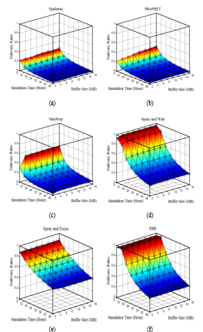Figure 1. Delivery ratio comparison: (a) Epidemic; (b) PRoPHET; (c) MaxProp. (d) SaW; (e) SaF; (f) EBR.

6.2. Impact of Varying the Traffic Load

Figure 3 shows the variation of delivery ratios as a function of message generation rate. One can notice that all protocols are negatively affected when the rate of message generation increases. In fact, in opportunistic networks with limited resources in terms of memory and energy, increasing the rate of the generation of the messages will increase traffic load, and consequently will increase both the dropping rate and the exchange of messages (i.e., transmission and reception of messages). This consumes the energy of the nodes. Over time, the number of dead nodes increases and becomes permanently out of service.

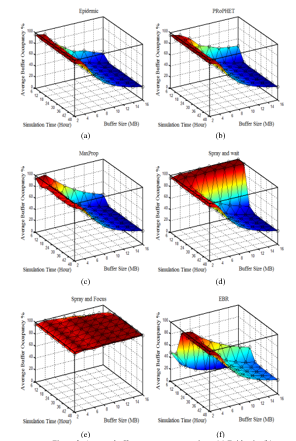Figure 2. Average buffer occupancy comparison: (a) Epidemic; (b) PRoPHET; (c) MaxProp. (d) SaW; (e) SaF; (f) EBR.

Figures 3 (a) – (f) show that the delivery ratio of the MaxProp, SaW, SaF, and EBR protocols, which use acknowledgements to delete redundant messages, is better than of the EPIDEMIC and PRoPHET. Thus, as shown in Figures 3 (a) and (b), both EPIDEMIC and PRoPHET achieve the best output ratio at the highest buffer value and the lowest traffic load at the coordinates point (7, 10). Conversely, they achieve the worst delivery ratio at the lowest buffer value and the highest traffic load, at the coordinates point (600, 2).

Figure 4 shows the effect of the traffic load on the overhead ratio. As mentioned earlier, the overhead reflects the cost of transmission in the network. Figures 4 (d) – (f) show that quota-based protocols have a high overhead when the message rate generation is high. This means that the transmission costs are high and the delivery ratio is low. This is confirmed by the Figures 3 (d) – (f). In general, as shown in Figure 4, the overload in the quota-based protocols is much lower than the overload in the flooding-based protocols.

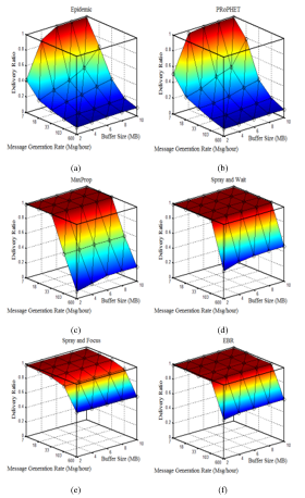Figure 3. Delivery ratio Comparison  for different traffic loads: (a) Epidemic; (b) PRoPHET; (c) MaxProp. (d) SaW; (e) SaF; (f)EBR.

Figures 4 (a) and (b) show that in the EPIDEMIC and PRoPHET protocols, at low levels of traffic load (i.e., 7, 18, and 33 Msgs / hour), the overhead gradually decreases as the buffer sizes increase, so the delivery ratio gradually increases too. This is confirmed by Figures 3 (a) and (b). However, unlike quota-based protocols, at high traffic load (that is 600 Msgs / hour) the overhead is low. The reason is that the high traffic load significantly affects the performance of the flooding-based protocols. Thus, the number of dead nodes increases resulting the decrease of the lifetime of the network. Hence, the overhead decreases.   From  the  results  given in Table II, at heavy traffic loads, both SaF and EBR have the highest delivery ratios, while SaF achieves the lowest overhead ratio and latency. On the other hand, the EPIDEMIC protocol exhibits the worst performance in terms of all the considered metrics.

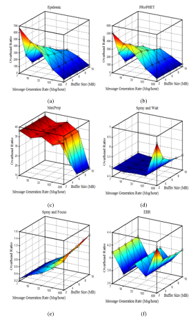Figure 4. Overhead ratio Comparison  for different traffic loads: (a) Epidemic; (b) PRoPHET; (c) MaxProp. (d) SaW; (e) SaF; (f)EBR.

6.3. Impact of Varying of number of nodes

Figure 5 shows that increasing the number of nodes while maintaining the rest of the parameters as listed in Table II, improves the delivery rate of quota-based routing protocols and greatly affects the delivery rate of flooding-based protocols. The reason is that in quota-based protocols, increasing the number of nodes increases the connectivity in the network and allows more messages to reach their destination. But, this will also lead to a large number of redundant messages that will roam the network and will drain its resources unless they are discarded. The inability to dispose of the redundant messages explains the low delivery ratio of the flooding-based protocols, as these messages will fill the buffers and will be frequently sent and received, which will drain nodes energy.

Figures 6 (a) – (f) depict the average latency time of the protocols. Obviously, the average latency at the nodes’ high density reaches its lowest value in all protocols. When the density of nodes is low, the average latency increases by increasing the buffer size. This is because message waiting times in the buffers increase, which in turn increases the delay.

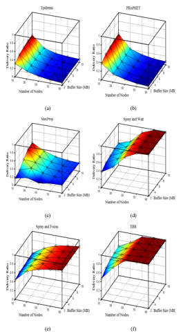Figure 5. Delivery ratio Comparison  for different number of nodes: (a) Epidemic; (b) PRoPHET; (c) MaxProp; (d) SaW; (e) SaF; (f) EBR.

As it shown from Figure 7, the overhead ratio increases in all protocols as the node density increases. This is due to the increase in the number of nodes that leads to an increase in connectivity among them. This in turn increases the relayed messages, and this causes the increasing in overhead ratio. From Figures 7 (a) and (b) we note that at the high density of the nodes, both protocols EPIDEMIC and PRoPHET are affected by buffer size. So that, the overhead decreases as buffer sizes increase.

Figure 5 shows that the EBR protocol achieves the best delivery ratio at the high node density. Figures 6 and 7 show that the SaF achieves the lowest overhead ratio and the lowest latency.

6.4. Impact of Varying of TTL

As presented in Table II, increasing message’ time to life (TTL) increases the delivery ratio, the overhead ratio, and the average latency. However, the results show that in flooding-based protocols, the overhead ratio and the average latency dramatically increase as the message life increases. This is because the messages remain in memory until the expiration time of the message.

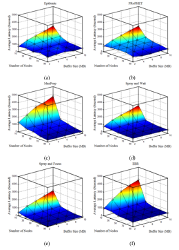Figure 6. Average latency Comparison  for different number of nodes: (a) Epidemic; (b) PRoPHET; (c) MaxProp; (d) SaW; (e) SaF; (f) EBR.

7. Design guidelines of routing protocols in the limited-resources Opportunistic Networks.

To design an effective routing protocol in resource-constrained opportunistic networks, the router should meet the following requirements: effective buffer management, impose an upper limit on message’ copies, skillful selection of messages on forwarding and deleting, skillful selection of the relay nodes by a utility-metric that includes the activity of the nodes and the contact history of the nodes.

Figure 7. Overhead ratio comparison  for different number of nodes: (a) Epidemic; (b) PRoPHET; (c) MaxProp. (d) SaW; € SaF; (f) EBR.

Based on the experiments results we deduce the following points:

• SaF routing protocol performs well in terms of all considered metrics against variations in traffic load and buffers size (see Section 6.2).
• SaF demonstrates superior performance in terms of overhead ratio and latency versus varying the density of nodes (see Section 6.3).
• EBR shows excellent performance in terms of delivery ratio against the variations in traffic load and density of nodes (see Sections 6.2 and 6.3).
• Quota-based routing protocols, which impose an upper limit on the number of messages’ copies in the network, outperform flooding-based and guided-flooding protocols.
• Guided flooding protocols, which have a mechanism to drive the message to its destination, outperform flooding-based routing protocols.
• In limited-resource environments, flooding-based routing protocols deplete network resources and cause the worst performance.

Based on the results of the analytical study and the study of the functioning of the SaF and EBR protocols, we recommend the following points when designing a routing protocol in opportunistic networks in resource-constrained environments:

• Use acknowledgments to eliminate duplicate messages. Surplus copies of the messages occupy large areas in buffers and are continuously sent and received in the network, draining the energy of the nodes and reducing its lifespan.
• Implement efficient buffer management. The mechanism used in buffer management plays an important role in performance. Efficient buffer management involves deciding which message to delete or send. This must be based on justifications imposed by the nature of the limited-resources environments.
• The choice of the next-hop should be based on precise estimation. When the node encounters other nodes, it must select the appropriate nodes for message forwarding. Message forwarding decision should ensure that the message reaches its destination at lowest cost and time.
• Using nodes’ contact history information to estimate forwarding decisions. Node’ contact history information reflects the mobility pattern of the node and can be used to estimate the node’s suitability to reach the message’s destination.
• Exploit active nodes in routing decisions. The preference of active nodes over others when making routing decisions increases the likelihood that the message will reach its destination. However, the estimation of node activity must be based on justifications associated with resource-limited environments, such as residual energy, buffer occupancy, and the number of node encounters.

8. Conclusion

In opportunistic networks, where communication among users is intermittent and resources are limited, it is difficult to reveal a strong statement about the kind of services offered by these networks. For this purpose, we identified the most important requirements that should be met in the routing protocols and give the best possible performance in such harsh environments. In this paper, we presented an analytical study on the performance of six of the most popular routing protocols in opportunistic networks namely: EPIDEMIC, PRoPHET, MaxProp, Spray and Wait, Spray and Focus and EBR. The results of the analysis showed that in order to design an effective routing protocol in resource-limited opportunistic networks, the router should effectively manage the buffer, set an upper limit on message copies, deftly select the messages on forwarding or deleting, and skillfully select the next hop based on a utility metric that includes the activity of the nodes and the contact history of the nodes.

Conflict of Interest

The authors declare no conflict of interest.

1. R. Nave, “Crossed Polarizers,” in Proceedings of the 2003 conference on Applications, technologies, architectures, and protocols for computer communications, 2012, pp. 27–34.
2. K. Hazra et al., “A Novel Network Architecture for Resource-Constrained Post-Disaster Environments,” in 2019 11th International Conference on Communication Systems and Networks, COMSNETS 2019, 2019, pp. 328–335.
3. N. Rajpoot and R. S. Kushwah, “An improved Prophet routing protocol for underwater communication,” in Proceedings of the 2015 international conference on communication networks (ICCN), 2016, pp. 27–32.
4. E. Max-Onakpoya et al., “Augmenting Cloud Connectivity with Opportunistic Networks for Rural Remote Patient Monitoring,” May 2019.
5. E. D. Ayele, N. Meratnia, and P. J. M. Havinga, “An Asynchronous Dual Radio Opportunistic Beacon Network Protocol for Wildlife Monitoring System,” 2019, pp. 1–7.
6. P. Liu, C. Wang, T. Fu, and Y. Ding, “Exploiting Opportunistic Coding in Throwbox-Based Multicast in Vehicular Delay Tolerant Networks,” IEEE Access, vol. 7, pp. 48459–48469, 2019.
7. P. Yuan, Z. Yang, Y. Wang, S. Gu, and Q. Zhang, “A Task-Driven Updated Discrete Graph Assisted Minimum Delivery Delay Routing for Remote Sensing Disruption-Tolerant Networks,” IEEE Access, vol. 7, pp. 69351–69362, 2019.
8. S. C. Nelson, M. Bakht, and R. Kravets, “Encounter-based routing in DTNs,” in Proceedings – IEEE INFOCOM, 2009, pp. 846–854.
9.  A. Vahdat and D. Becker, “Epidemic routing for partially connected ad hoc networks,” 2000.
10. T. Abdelkader, K. Naik, A. Nayak, N. Goel, and V. Srivastava, “A performance comparison of delay-tolerant network routing protocols,” IEEE Netw., vol. 30, no. 2, pp. 46–53, Mar. 2016.
11.  A. Lindgren, A. Doria, and O. Schelén, “Probabilistic Routing in Intermittently Connected Networks,” 2004, pp. 239–254.
12. J. Burgess, B. Gallagher, D. Jensen, and B. N. Levine, “MaxProp: Routing for vehicle-based disruption-tolerant networks,” in Proceedings – IEEE INFOCOM, 2006.
13.  T. Spyropoulos, K. Psounis, and C. S. Raghavendra, “Efficient Routing in Intermittently Connected Mobile Networks: The Multiple-Copy Case,” IEEE/ACM Trans. Netw., vol. 16, no. 1, pp. 77–90, Feb. 2008.
14.  T. Spyropoulos, K. Psounis, and C. S. Raghavendra, “Spray and focus: Efficient mobility-assisted routing for heterogeneous and correlated mobility,” in Proceedings – Fifth Annual IEEE International Conference on Pervasive Computing and Communications Workshops, PerCom Workshops 2007, 2007, pp. 79–85.
15. S. Palazzo, A. T. Campbell, and M. Dias de Amorim, “Opportunistic and Delay-Tolerant Networks,” EURASIP J. Wirel. Commun. Netw., vol. 2011, no. 1, p. 164370, Dec. 2011.
16. A. Socievole, F. De Rango, and C. Coscarella, “Routing approaches and performance evaluation in delay tolerant networks,” in Wireless Telecommunications Symposium, 2011.
17. M. S. Hossen and M. S. Rahim, “Performance evaluation of replication-based DTN routing protocols in Intermittently Connected Mobile Networks,” in ICEEE 2015 – 1st International Conference on Electrical and Electronic Engineering, 2016, pp. 101–104.
18. V. N. G. J. Soares, J. J. P. C. Rodrigues, J. A. Dias, and J. N. Isento, “Performance analysis of routing protocols for vehicular delay-tolerant networks,” in 2012 20th International Conference on Software, Telecommunications and Computer Networks, SoftCOM 2012, 2012.
19. A. Socievole and F. De Rango, “Evaluation of routing schemes in opportunistic networks considering energy consumption,” in Simulation Series, 2012, vol. 44, no. BOOK 12, pp. 41–47.
20. M. Alajeely, A. Ahmad, and R. Doss, “Comparative study of routing protocols for opportunistic networks,” in Proceedings of the International Conference on Sensing Technology, ICST, 2013, pp. 209–214.
21. N. Chakchouk, “A Survey on Opportunistic Routing in Wireless Communication Networks,” IEEE Commun. Surv. Tutorials, vol. 17, no. 4, pp. 2214–2241, Oct. 2015.
22. J. Cui, S. Cao, Y. Chang, L. Wu, D. Liu, and Y. Yang, “An Adaptive Spray and Wait Routing Algorithm Based on Quality of Node in Delay Tolerant Network,” IEEE Access, vol. 7, pp. 35274–35286, 2019.
23. A. Keränen, J. Ott, and T. Kärkkäinen, “The ONE simulator for DTN protocol evaluation,” in SIMUTools 2009 – 2nd International ICST Conference on Simulation Tools and Techniques, 2009.
24. “The ONE.” [Online]. Available: https://www.netlab.tkk.fi/tutkimus/dtn/theone/. [Accessed: 26-Nov-2019].

(Click Here)

(Click Here)