1. Introduction

Nowadays, automation is playing an increasingly important role in our daily lives, therefore is a growing need for the autonomous motion-planning of robotic manipulators.

Two types of path-planning methods can be defined, the offline and the online methods. In case of offline path-planning method, the calculation time does not mean a bottleneck, so more time can be spent on improving the found path. For example, in [1] an offline path-planning method is introduced, that can find an optimal collision-free path, where the optimality is based on the energy usage of the manipulator. These kind of methods can ensure the collision-freeness only with static obstacles or obstacles with known motions.

Online path-planning methods are used to avoid collisions with dynamic obstacles having unpredictable movements. These algorithms can be used in human-robot collaboration systems for example [2]. The environment of the robot can be observed with a depth camera. Besides, the image processing can be calculated with GPU, so the real-time calculation can be ensured [3]. In this paper, an offline path planning method will be described.

In our case, the minimization of cost-function is needed during the motion-planning algorithm, while avoiding configurations leading to collisions. There are numerous solutions in robotic applications to this problem.

Many of these are founded on the classical grid-based methods like A* or D* which can be used to find an optimal path limited by the resolution of the grid [4]. The main disadvantage of these algorithms is that the computation time grows exponentially with the number of dimensions. This effect is called as the “Curse of dimensionality”.

Another type of path-planning methods are the sampling-based algorithms like the Rapidly-exploring Random Tree (RRT). These algorithms can be used effectively with higher number of dimensions as well, but the optimality of the solution is not guaranteed [5].

These problems can be solved by the Transition-based RRT (TRRT) algorithm, that incorporates the advantages of the grid-based and the sampling-based methods [6]. Thus, it can be used to find a path that minimizes a cost-function defined in the high dimensional search space.

Heuristics can be used to determine the meaning of cost. For example, in case of a human-collaboration, to ensure the safe operation and the security, the cost has to be high near by the person [7].

Another method could be that, when the dynamics of the system is used to minimize the time or the performed work during the motion.

In this paper, the goal is to maximize the distance between the path of the manipulator and the configurations that cause collisions with the help of defined cost function. In this case the result of the offline path-planning algorithm can be used by a reactive motion planning method, that will have more space to avoid dynamic obstacles.

The paper is organized as follows. Section 2 introduces the base of the kinematics of robotic manipulators. In Section 3, the T-RRT algorithm is presented, that was used for path-planning in this work. Then the collision-detection method is described, based on investigation of the feasibility of inequalities of bounding polyhedra, that are describing the manipulator and the obstacles (Section 4). Then, Section 5 describes two cost function approximation algorithms with Gauss-functions and with fuzzy function-approximation. The latter is more detailed. Subsection 5.5 describes the method that is used in this work for cost function evaluation. The trajectory generation method is explained in Section 6. The simulation results are presented in Section 7. Finally, Section 8 contains conclusions and possible developments in the future.

2. Robotic manipulators

Robotic manipulators are usually modeled as open kinematic chains. A manipulator contains links, which are connected by joints. Two basic types of joints exist: Revolute joints are used to apply relative rotation, and prismatic joints allow linear motion between two adjacent links. The relative movement between adjacent links is given by the joint variables q_i. In case of revolute joints, q_i gives the angular displacement, while for prismatic joints, q_i equals the amount of linear motion. The actual configuration q of the robot is defined by the vector containing actual q_i values of all joints.

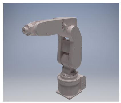Figure 1: Mitsubishi RV-2F-Q manipulator (used in the simulations)

An end effector is usually attached to the last segment of the manipulator. To determine the position and the orientation of the end effector in the workspace of the robot, the equations of forward kinematics can be used. A homogeneous transformation matrix belongs to each robotic joints. The position and orientation of the coordinate frame attached to the end effector (relative to the base frame) can be determined by multiplying these matrices.

The main parameters of a robotic manipulator can be defined by the Denavit-Hartenberg parameters [8]. Homogeneous transformation matrices can be calculated from these parameters using actual joint variables.

The task of the path-planning is to find a path, which moves the robot to a desired goal configuration. (This goal configuration is typically given by the desired orientation and position of the end-effector at the end of the motion.) The path-planning problem can be defined in the Euclidean space, but usually, the planning is performed in the configuration space C of robot. The configuration space is spanned by the admissible configuration vectors (q), i.e. joint variables (q_i) are used as coordinates. For example the configuration space of the Mitsubishi RV-2F-Q manipulator with six degrees of freedom is a six-dimensional space. This robot has six revolute joints. Its 3D model is depicted in Fig. 1. The simulations presented in Section 7 were performed using this manipulator.

3. The Path-planning Algorithm

The traditional RRT algorithm is a stochastic sampling pathplanning algorithm. In this method a search tree is grown from the initial q_init point to the q_goal goal configuration. In a given iteration, a randomly selected configuration is inserted to the tree [9].

In these days, the planning algorithms like the RRT method are very popular, due to their efficiency in exploration of the search space. There exist several improvements of the traditional method, for example the RRT* described in [10], which checks the available corrections in every iteration cycle, so it is able to find an optimal path to the goal point. The method presented in [11] called RRT⁺ can be used in very high dimensional spaces, such as the configuration space of hyper-redundant manipulators. In this work, the T-RRT algorithm is used, that is able to find a suboptimal solution defined by a cost function in high dimensional configuration spaces as well. This solution is called as high quality path in [6]. In our case the goal of cost function is to minimize the risk of collision.

Algorithm 1: Rapidly-exploring Random Tree (RRT)

Input: the configuration space C the root q_init and the goal q_goal

Output: the tree T

1: T ← InitTree(q_init)

2: while not StopCondition(T,q_goal) do 3: q_rand ← SampleConf(C)

         4:        q_near ← NearestNeighbor(q_rand,T)

         5:         qnew ← Extend(T,qrand,qnear)

         6:        if NoCollision(q_new) then

7:    AddNewNode(T,q_new) 8:      AddNewEdge(T,q_near,q_new)

         9:       end if

10: end while

11: return T

In Algorithm 1 the traditional RRT algorithm is described. The inputs of the algorithm is the configuration space, where the pathplanning method is evaluated, the initial and the goal configuration of the path-planning. The output of the method is the search tree. At first, the search tree is initialized with the initial configuration as its root node.

After that a uniformly distributed random configuration q_rand is generated in function SampleConf.

This configuration is used by the NearestNeighbor function to determine the nearest configuration (called q_near) to it in the search tree. In this method, distance from the edges is not examined, due to the higher computational demand, it is determined only from the previously added nodes.

A new point q_new is created in Extend, which is in the same direction as q_rand to q_near, but the distance between q_new and q_near is maximized with the parameter δ. In this method, the collision-

freeness of the created q_new configuration is not examined.

The function NoCollision returns true, if the q_new configuration does not lead to a collision. In this case, a new node and edge will

be added to the tree.

The algorithm is succeeded, if the distance between the last inserted point and the goal configuration is less than a given parameter, or failed, if a maximum number of iterations has been reached. In the function StopCondition are these conditions inspected.

Algorithm 2 describes the T-RRT method. As it can be seen, the method is based on the traditional RRT algorithm described in Algorithm 1. The main differences are the TransitionTest and MinExpandControl functions (see Subsections 3.1-3.2), which are the conditions to extend the search tree with a new node and edge.

The cost of the found path can be evaluated by several methods, e.g. maximal cost, average cost or total cost along the path. However it will lead to a path, that avoids the areas of search space with higher costs, if the performed work is minimized along the path, as it is introduced in [6]. In this case, the positive variations of the cost function will be minimized.

Algorithm 2: Transition-based RRT

Input: the configuration space C the cost function c : C 7→ R^∗₊

the root q_init and the goal q_goal

Output: the tree T

1: T ← InitTree(q_init)

2: while not StopCondition(T,q_goal) do

         3:        q_rand ← SampleConf(C)

         4:        q_near ← NearestNeighbor(q_rand,T)

         5:         qnew ← Extend(T,qrand,qnear)

         6:         if q_new , NULL then

         7:            dnear−new ← Distance(qnear,qnew)

8:           if TransitionTest(c(q_near),c(q_new),d_near−new) and MinExpandControl(T,q_near,q_rand) and NoCollision(q_new) then

         9:                AddNewNode(T,q_new)

        10:                AddNewEdge(T,q_near,q_new)

        11:           end if

        12:       end if

13: end while

14: return T

3.1        Transition-test

Algorithm 3 describes the TransitionTest function. In the first step, the number, how many times the transition-test failed previously, is queried by the GetCurrentNFail function.

Thereafter if the cost in q_new point is higher than a c_max parameter, then the test will not be accepted, so the search tree will not be extended. In case of negative variation of cost function the transition test will return true.

After that in case of positive slope of the cost, the transition test will be successful in accordance with a probability based on the

Metropolis criterion [12], defined as

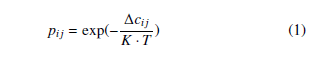where ∆c_ij = _dij is the variation of the cost, K is a normalization constant, it can be taken as the average cost of the query configurations.

The difficulty of success for a given transition is defined by the temperature parameter denoted by T. The goal of this parameter is to minimize the amount of positive slopes in the cost function along the path, but it allows to explore the whole reachable configuration space by its adaptive tuning. In case of higher temperature the acceptance of transition test is more probable for a transition with higher positive slope. To accept only very low positive variations at the start, T is initialized with a very low value. This functions similar to the simulated annealing algorithm.

The function Rand(0,1) gives a random number between 0 and 1 based on uniform distribution.

The α > 1 variable is used to change the temperature adaptively. If the transition was successful then the temperature is decreased. And if the test failed nFail_max times then the value of T is increased by multiplying with α. Thus if the nFail_max parameter is high then the path will be more likely to go into the valleys, however finding a path over a region with high cost will be more difficult.

Algorithm 3: TransitionTest(c_i,c_j,d_ij)

1: nFail = GetCurrentNFail();

2: if c_j > c_max then

          3:        return False

4: end if

5: if c_j < c_i then

          6:        return True

7: end if

−(cj−ci)/dij

           8: p = exp( K·T                        )

9: if Rand(0, 1) < p then

        10:        T = T/α

        11:        nFail = 0

        12:        return True

13: else

        14:         if nFail > nFail_max then

        15:            T = T · α

        16:            nFail = 0

        17:      else

        18:             nFail = nFail + 1

        19:       end if

        20:        return False

21: end if

3.2        Minimal Expansion Control

The transition-test can slow the exploration rate of high cost hills and the new configurations only refine the already known regions.

By specifying a minimum level of exploration, this can be prevented. Accordingly, a new node close to the closest search tree configuration will only be accepted if the refining node ratio is smaller than the ρ parameter. The minimal exploration control method will accept the exploring nodes automatically.

This function is introduced in Algorithm 4. The function UpdateNbNodeTree increases the number of nodes, while the UpdateNbRefineNodeTree function updates the number of refining nodes in the search tree.

The Euclidean distance between the q_rand (not the extended q_new) and the q_near configurations is used to determine the type of a given point. A point is an exploring node if the distance is high, otherwise it will be a refining node.

The path-planning will discover the entire configuration space very effectively with this complement, while trying to stay in the valleys of the cost function owing to the transition-test.

Algorithm 4: MinExpandControl(T,q_near,q_rand)

1: if Distance(q_near,q_rand) > δ then

         2:       UpdateNbNodeTree(T)

         3:        return True

4: else

         5: if NbRNefinebNodeNodeTreeTree(T+(T1)+1) > ρ then

         6:            return False

         7:       else

         8:           UpdateNbRefineNodeTree(T)

         9:           UpdateNbNodeTree(T)

       10:            return True

       11:       end if

12: end if

4. Collision detection

The effectiveness of a path planning method depends highly on the applied collision detection function, since it is called often (see Step 6 of Algorithm 1 or Step 8 of Algorithm 2) and it has to ensure that only collision-free configurations are used for planning. To calculate in real time, which robot configurations are in collisions, is a difficult problem. The task is not only to determine if there is any collision between the robot and the surrounding objects, but also the self-collision configurations of the robot has to be avoided.

Moreover, the goal could be not only to plan a collision-free path, but also to get a time-optimal motion. A solution for such a problem is presented in [1], but the computational demand of that algorithm is high, due to the solution of the optimization problem. However, the collision detection algorithm used by that method can be applied by other applications as well. The algorithm presented in this paper is also based on this collision detection.

4.1        Collision detection with polyhedrons

The basic idea of this collision detection method is that the geometry of the robot and the obstacles is approximated such that they are represented by unions of convex polyhedrons. Fig. 2 and Fig. 3 illustrate how the bounding polyhedrons can be determined around the robot and the obstacles. For the sake of simplicity, it is supposed that the workspace of the robot contains only one obstacle. The presented collision detection method can be easily extended if more obstacles are present.

Let P denote the union of polyhedrons that represent the robot:

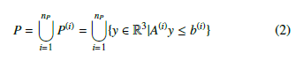where n_P shows the number of polyhedrons in P. A polyhedron is bounded by faces. A face P⁽ⁱ⁾ is defined by A⁽ⁱ⁾ and b⁽ⁱ⁾ parameters and p_i is the number of faces. Then A⁽ⁱ⁾ ∈ R^pi×3 and b⁽ⁱ⁾ ∈ R^pi for i = 1,…,n_p.

Similarly, an obstacle Q can also be described by the union of polyhedrons:

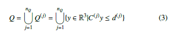where n_Q denotes the number of polyhedrons in Q. q_j shows the number of faces in Q^(j), hence C^(j) ∈ R^qj×3 and d^(j) ∈ R^qj for j = 1,…,n_Q.

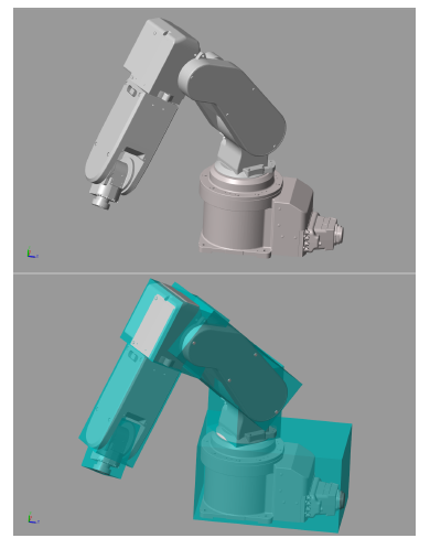Figure 2: Bounding boxes of each segments were defined as the bounding polyhedrons of the manipulator

To avoid self-collisions, pairs of polyhedrons P⁽ⁱ⁾ have to be checked, whether they collide with each-other. There exist such pairs of P⁽ⁱ⁾ where the collision detection is not necessary, since they cannot collide physically (e.g. adjacent segments). Therefore, the set of pairs (k,l), k , l has to be defined, such that k and l denote two polyhedrons (P^(k), P^(l)) of the robot which could collide. This set is denoted by I. If (k,l) ∈ I, the collision check has to be performed for the corresponding two polyhedrons.

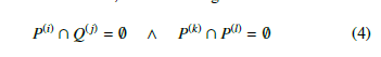
Suppose, that P is already calculated for a given configuration and Q is determined as well, then the configuration is collision-free if

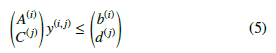
One polyhedron of the robot P⁽ⁱ⁾ and one of the obstacle Q^(j) do not collide with each-other if the union of their system of inequalities has no solution. Formally, there exists no such y^(i,j) ∈ R³ point where

Similar inequalities can be used to check self-collision.

To determine, whether an inequality similar to (5) has no solution, Farkas’s lemma can be applied. The lemma says that there exists no solution for the linear system if and only if a vector

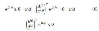Consequently, if given is a configuration q and a w^(i,j) solution can be found for (6), then the q configuration can be marked as collision-free.

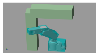Figure 3: Bounding polyhedrons around the robot and obstacles (as used in the simulation)

4.2        Construction of polyhedrons

The face parameters (A⁽ⁱ⁾,b⁽ⁱ⁾) for some robot-polyhedron P⁽ⁱ⁾ depend on the actual robot configuration q. This subsection describes how to calculate them.

First, A⁽_rⁱ⁾ and b⁽_rⁱ⁾ have to be determined for each segment of the robot in a reference coordinate system that is attached to the same segment. For example, the CAD model of the manipulator (e.g. shown in Fig. 1) can be used to measure the corresponding parameters in this frame. (For obstacles, the same process has to be performed.)

Then, a transformation is required to get these parameters in the base frame. Denote the resultant transformation matrix by T⁽ⁱ⁾(q). T⁽ⁱ⁾(q) can be used for the transformation from the base coordinate system to the reference frame of the i_th segment, if the actual configuration of the robot is q.

The parameters in the base frame can be determined as follows

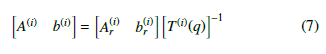During the collision-check algorithm, these parameters have to be used.

5. Cost-function approximation

The goal of cost-function is to keep distance from configurations leading to a collision. The approximation of this function is necessary, to decrease the computational demand of the algorithm. This cost-function is used by the T-RRT path-planning method, introduced in Section 3.

5.1        Cost-funcion approximation with Gauss-functions

At first, the approximation of cost-function was evaluated by taking enough sample of the configuration space and Gauss-functions were summed in every sampling point. The centers of Gauss-functions are the configurations causing a collision. There are several disadvantages of this method.

As it can be seen in the Fig. 4 the result is very hilly and a maximal value of the cost function can not be predefined, so the c_max parameter of the TransitionTest function in Algorithm 3 is difficult to determine.

In addition, the cost function has to be stored in every sampling point, moreover the interpolation is slow at any other point.

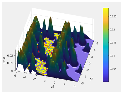Figure 4: Cost-function approximation with Gauss-functions with the search tree

found by the T-RRT algorithm

5.2        The base of fuzzy approximation

Another solution could be the fuzzy approximator systems.

Fuzzy systems have several uses in many areas such as decision making [13], system identification [14], control theory [15] etc. In addition, the approximation of nonlinear functions is possible as well, if enough teaching points are available. Teaching points are defined as y_j = f(x_j), where f is the function that needs to be approximated, x_j is the position of the given teaching point and y_j is the value of f in x_j.

There are several advantages of fuzzy estimator systems. Depending on which type of inference method is used, their rules can be tuned adaptively and the approximation time is one of the benefits of these systems as well.

Singleton fuzzyfication, center average defuzzyfication, product inference and zero-order Sugeno model fuzzy systems with Gaussian membership functions are therefore the most widely used approaches [16].

Thus the fuzzy estimation of a nonlinear function is defined as

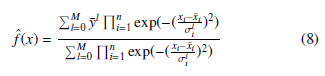where n is the number of dimensions in the configuration space, y¯^l is the output in the l_th rule of the fuzzy inference system, x¯_i is the location of the maximum value of the Gaussian membership function and with σ^l_i the width of this function can be modified.

The adaptive tuning of the fuzzy rules is feasible by modifying the ¯y^l, ¯x_i and σ^l_i values.

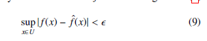
According to the Universal approximation theorem described in [16], for any given real continuous function f on the compact set U ∈ Rⁿ and arbitrary  > 0 there exists fˆ in the form given in (8) such that

Henceforth, two adaptive tuning method for fuzzy estimator systems will be introduced. In which bounded domain intervals of input vector x and output y are assumed.

5.3        Generating fuzzy rules by learning from examples

Details of the algorithm can be found in [17].

The input and output domain is divided into intervals, in each Gaussian membership functions are defined.

The possible fuzzy relations are determined exactly by the number of input membership functions. For example, in case of input variables x₁ and x₂, if the number of membership functions are N₁ and N₂ then the number of possible rules is N₁ · N₂. For each teaching point the relation and output membership function has to be selected that mostly fits the given teaching point.

In k_th teaching step a generic form of fuzzy rules can be defined:

where F_i^k is one of the input variable membership functions and G^k is one of the output variable membership functions.

In the k_th step a given rule will be chosen, if it maximizes the following expression:

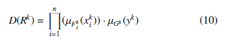where µ is the firing strength of the given membership function for the actual value of the teaching point.

There exist more possible solutions to that problem, if a new relation has to be added with the same condition part, but a different inference part as an already added relation. In this case, the relation with higher value can be selected by evaluating (10), or a weighted value of both inference parts can be specified.

The main disadvantage of this technique is that (10) has to be evaluated N = N₁ · N₂ · … · N_n times for every teaching points (where n is the number of dimensions of the space) to find the maximum value. As a consequence, with the number of dimensions the computational time grows exponentially.

5.4        Nearest neighborhood clustering

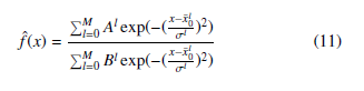
In this algorithm, teaching points are clustered depending on their position in the configuration space. A given cluster can be described by three parameter, the center of it x₀^l , the number of teaching points in it B^l and the sum of values of these points A^l [18].

A new point x_j (y_j = f(x_j)) is inserted to the cluster l, if it is closer to x₀^l than a given r radius. After that the other cluster parameters A^l and B^l will be updated. If the distance of the teaching point x_j is too high from all of the clusters then a new cluster will be created as {x₀^l = x_j; A^l = y_j; B^l = 1}. M represents the number of clusters that have been defined during the teaching process.

Therefore, the estimation of the nonlinear function can be defined as

5.5        Cost-function evaluation

Eventually, the cost-function for the T-RRT method was approximated with the Nearest neighborhood clustering algorithm, because it has a higher computational efficiency.

To determine the position of the teaching points, random sampling of the configuration space is needed, owing to the high number of dimensions.

The collision detection method described in Section 4 is evaluated in all of teaching points. If the x_j configuration causes collision, then one will be assigned as the value of the cost-function y_j in x_j, otherwise zero.

After that the rules of the fuzzy approximator are tuned with the Nearest neighborhood clustering algorithm. This method can be used for arbitrary robotic manipulators. An example for the cost function and path can be seen in Fig. 5 in case of 2-DoF manipulator (since it is not possible to depict the cost function in higher dimensions).

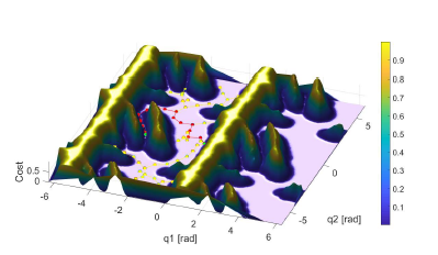Figure 5: T-RRT method is able to find high quality path based on a cost-function.

The cost-function is evaluated for a two degrees of freedom manipulator with the Nearest Neighborhood Clustering algorithm.

Table 1 shows the comparison of approximation with Gaussfunction and the Nearest neighborhood clustering algorithm. As can be seen, both the training time and the evaluation time for one configuration in the case of Gauss-function approximation grow very fast by increasing the number of teaching points. In the case of Nearest neighborhood clustering, these values increased to a lesser extent. By using clusters, the evaluation time of the fuzzy functionapproximation method did not increase significantly, which is ideal for applying the method in a path-planning algorithm.

Table 1: Comparison of fuzzy function-approximation and approximation with

1000	0.0481s	714	22µs	0.0402s	7.8µs
5000	0.207s	1649	45µs	0.3027s	28.8µs
10000	0.4554s	1974	52µs	1.4151s	58.2µs
50000	3.0962s	2431	65µs	22.88s	137.9µs
100000	7.045s	2521	76µs	155.26s	1632µs

Num. of teaching	Nearest Neighborhood clustering			Gauss
	Training	Number	Eval.	Training	Eval.
points	time	of clusters	time	time	time

Gauss-functions

6. Trajectory generation

The already presented methods can be used to find points in the configuration space, that by moving the robot between these points, the possible collisions can be avoided.

6.1        Trajectory generation for scalar values

In the following method y denotes one coordinate of the q configuration, in other words, one joint variable of the robot.

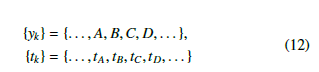
Let {y_k} be the set of points founded by the path-planning algorithm and {t_k} denotes the desired absolute time of reaching these points [19].

Due to the limits of torques, boundaries have to be defined for the acceleration of joints: |y¨|_max.

At first, y(t) trajectory can be defined as a series of linear functions between adjacent points. In this case, the first derivative y˙(t) is constant between two points and it steps to another constant value in a given point. The acceleration y¨(t) is zero in every point except the points where the slope of y(t) trajectory is changing. In these points, the second derivative contains Dirac-delta functions, which leads to an unbounded control value, so this solution is not applicable. To overcome this problem, the acceleration of joints have to be changed continuously.

To reach the next point two kinds of phases can be defined: traveling phase and acceleration phase. In the former, we use a constant velocity and zero acceleration, while in the latter a continuous acceleration function has to be applied, to reach the desired constant velocity of the next traveling phase. The quadratic function can be chosen as the form of the function in the acceleration phase (Fig. 6).

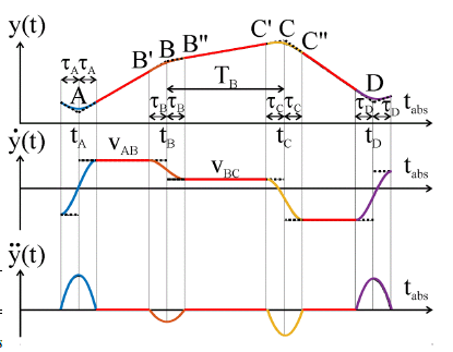Figure 6: To ensure the continuity of the acceleration function, quadratic function can be applied in the acceleration phase. The form of the trajectories can be seen in the figure.

Let B and C be two adjacent points, while B⁰ and C⁰ are the beginning, B⁰⁰ and C⁰⁰ are the end of their acceleration phase. The relative time t can be defined as

where t_B is the absolute time of reaching the point B, τ_B is the half of duration of acceleration phase in B and T_B denotes the time-interval of reaching point C from point B. This can be seen in Fig 7. The time-intervals between configurations can be determined by the boundaries of joint-velocities, for example T_B ⁼ _|^C_y˙|⁻max^B .

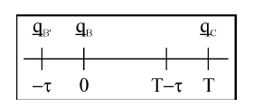Figure 7: Relative time can be defined, where the zero value is in the q_B configuration.

The zero point will be shifted with T, when the T −τ relative time is reached.

By integrating the quadratic acceleration during the acceleration phase, the velocity and position can be determined:

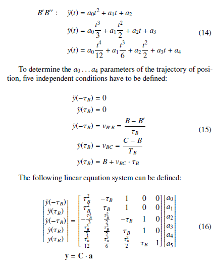The solution of this linear equation system can be calculated as follows:

6.2        Trajectory generation for joint variables

The presented method for scalar values can be used for each joint variable separately, by taking into account the difference between the boundaries of velocities (|q˙_i|_max) and accelerations (|q¨_i|_max) of some joints.

In addition, the minimal time needed to reach q_Ci joint value from q_Bi can be different as well, so just that joint have to be moved in maximal speed, that needs the most time to reach the next configuration.

The same τ parameter can be used for each joint variable and it is calculated as follows [19]:

The trajectory generation method can be seen in the Algorithm 5. The input of the method denoted by Q is the series of configurations contained by the found path.

Algorithm 5: TrajectoryGeneration(Q,τ)

1: qC =GetFirstConfiguration(Q) 2: T = τ 3: while Size(Q) > 0 do
4:	qB0 = q(T − τ)
5:	qB = qC
6:	qC = GetFirstConfiguration(Q)
7:	Ti = |q|Ciq˙i−|maxqBi|
8:	T = max{max{Ti},2τ} i
9: 10:	vAB = qB−τqB0 vBC = qCT−qB
11:	a = C−1 · y
12:	t = −τ
13:	while t < T − τ do
14:	q(t) = CalculateTrajectory(a,t)
15:	t = t + ∆
16:	end while
17: end while 18: return q(t)

The GetFirstConfiguration function gives the first element of the configuration queue and this element will be removed from the queue as well.

At first the variable T is initialized with τ calculated by (19), so in the first iteration the q_B0 variable will be the root configuration.

The equations in (14) are evaluated in the CalculateTrajectory function for each joint variable, consequently the dimension of the q variable is equal to the dimension of the configuration space.

Trajectories calculated with this method can be seen in Fig. 9.

7. Simulation results

The comparison of several path-planning algorithms can be seen in Table 2 in case of two degrees of freedom robotic manipulator. The result of planning with the T-RRT method can be seen in Fig. 8. The RRT^∗ algorithm is a variant of traditional RRT method, that refines the search tree in every iteration to find the actual shortest path to the goal configuration [10]. In case of multi-directional RRT method an other search tree is started from the goal configuration [5]. The calculation time can be reduced by this method.

Table 2: Comparison of path-planning algorithms

                                       Calculation                        Total       Performed

Algorithm                Length time [s]          cost         work

RRT	0.039	10.54	0.415	0.896
Multi-directional RRT	0.019	10.54	0.396	0.822
Multi-directional RRT∗	3.34	6.92	0.171	0.449
T-RRTg	0.55	10.21	0.028	0.121
T-RRTt	13.466	10.91	0.01	0.062

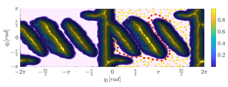Figure 8: The result of path-planning for two degrees of freedom manipulator with the tempered version of T-RRT

Two parameter settings are examined for the T-RRT method, the first one (T-RRT_g) is a greedy version with nFail_max = 10, in the other case (T-RRT_t) nFail_max = 100, which will lead to a tempered version of T-RRT. The computation time in the first case is lower, but the found path has a lower quality as well. The other parameters were: T_init = 10⁻⁵, α = 1.5, ρ = 0.2, c_max = 0.4, δ = 0.3. The parameters were chosen empirically.

As it can be seen, the path of the T-RRT algorithm is not equal with the shortest collision-free path.

To demonstrate the presented method, simulations were performed using the Mitsubishi RV-2F-Q manipulator as well. The task of the robot was to move to the other side of an obstacle, which is modeled by two polyhedrons. For implementation and simulation, MATLAB Simulink and Simscape Multibody toolbox were used. The running times were measured on a computer with Intel Core i7-7700HQ Processor.

For the cost function evaluation, the nearest neighborhood clustering method was applied. The parameters were empirically selected as follows: number of teaching points is n = 20000, radius of the cluster is r = 1 rad and deviation of the Guassian membership functions is σ = 0.5. To determine the approximated cost function, t ≈ 120s computational time was required, what is appropriate, since these calculations have to be performed only once for a given robot and workspace.

The parameters of the T-RRT method were selected as T_init = 0.01, α = 5, nFail_Max = 10, ρ = 0.1, c_max = 0.8 and δ = 0.4. To get a solution for a path-planning problem, the average calculation time was t ≈ 7.3s.

One solution is presented in Fig. 9–Fig. 10. Fig. 9 depicts the trajectories of the joint variables. The whole movement can be seen in a video: https://youtu.be/t6GO8LKG5js. Some key configurations of the robot are also presented in Fig. 10. It can be seen, that the presented algorithm was able to plan such a motion, where colliding configurations can be avoided.

8. Conclusion

The method presented in this paper can be used to solve the offline path-planning problem for robotic manipulators. The algorithm is based on the T-RRT method, which is able to calculate the reference motion for the robot, such that collision avoidance is guaranteed and suboptimal path is selected according to some cost-function.

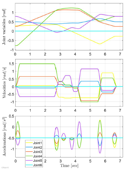Figure 9: Trajectories of the joint variables

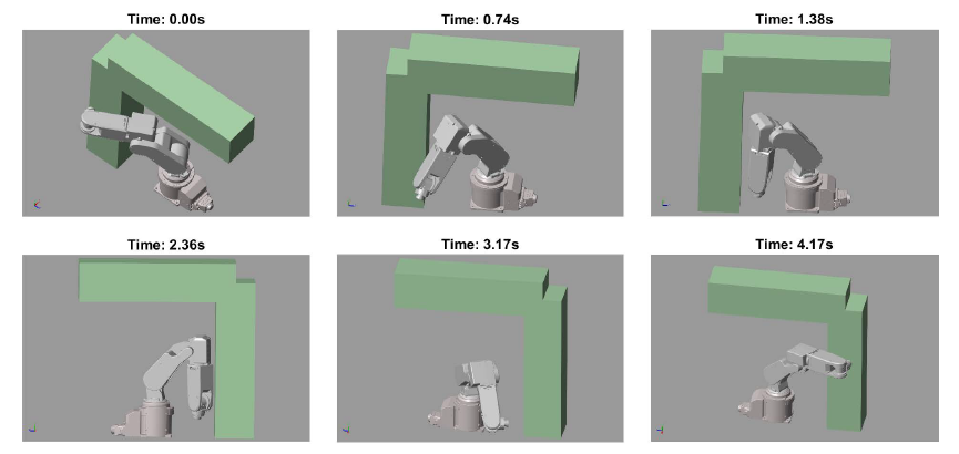Figure 10: Robot configurations along the collision-free path

1. Chantal Landry, Matthias Gerdts, Rene´ Henrion, and Dietmar Ho¨mberg. Path- planning with collision avoidance in automotive industry. In IFIP Conference on System Modeling and Optimization, pages 102–111. Springer, 2011.
2.  Fabrizio Flacco, Torsten Kro¨ ger, Alessandro De Luca, and Oussama Khatib. A depth space approach to human-robot collision avoidance. In 2012 IEEE International Conference on Robotics and Automation, pages 338–345. IEEE, 2012.
3. Massimo Cefalo, Emanuele Magrini, and Giuseppe Oriolo. Parallel collision check for sensor based real-time motion planning. In 2017 IEEE International Conference on Robotics and Automation (ICRA), pages 1936–1943. IEEE, 2017.
4. Anthony Stentz. Optimal and efficient path planning for partially known envi- ronments. In Intelligent Unmanned Ground Vehicles, pages 203–220. Springer, 1997.
5. Steven M LaValle. Planning algorithms. Cambridge University Press, 2006.
6. Le´onard Jaillet, Juan Corte´s, and Thierry Sime´on. Sampling-based path planning on configuration-space costmaps. IEEE Transactions on Robotics, 26(4):635–646, 2010.
7. Ran Zhao. Trajectory planning and control for robot manipulations. PhD thesis, Universite´ Paul Sabatier-Toulouse III, 2015.
8. Mark W Spong, Seth Hutchinson, Mathukumalli Vidyasagar, et al. Robot modeling and control. John Wiley & Sons, Inc., 2006.
9. Steven M LaValle. Rapidly-exploring random trees: A new tool for path planning. Technical report, Department of Computer Science, Iowa State University, 1998.
10. Sertac Karaman and Emilio Frazzoli. Sampling-based algorithms for optimal motion planning. The international journal of robotics research, 30(7):846– 894, 2011.
11. Marios Xanthidis, Ioannis Rekleitis, and Jason M O’Kane. Rrt+: Fast planning for high-dimensional configuration spaces. arXiv preprint arXiv:1612.07333, 2016.
12. Peter JM Van Laarhoven and Emile HL Aarts. Simulated annealing. In Simulated annealing: Theory and applications, pages 7–15. Springer, 1987.
13. Dug Hun Hong and Chang-Hwan Choi. Multicriteria fuzzy decision-making problems based on vague set theory. Fuzzy sets and systems, 114(1):103–113, 2000.
14. Robert Babuska and Henk Verbruggen. Neuro-fuzzy methods for nonlinear system identification. Annual reviews in control, 27(1):73–85, 2003.
15. L-X Wang. Stable adaptive fuzzy control of nonlinear systems. IEEE Transactions on fuzzy systems, 1(2):146–155, 1993.
16. L-X Wang. Fuzzy systems are universal approximators. In [1992 Proceedings] IEEE International Conference on Fuzzy Systems, pages 1163–1170. IEEE, 1992.
17. L-X Wang and Jerry M Mendel. Generating fuzzy rules by learning from exam- ples. IEEE Transactions on systems, man, and cybernetics, 22(6):1414–1427, 1992.
18. L . Wang. Training of fuzzy logic systems using nearest neighborhood cluster- ing. In [Proceedings 1993] Second IEEE International Conference on Fuzzy Systems, pages 13–17 vol.1, March 1993.
19. Lantos Be´la. Robotok ir ́any ́ıt ́asa (Robot Control). Akade´miai K., 2002.
20. MG Mohanan and Ambuja Salgoankar. A survey of robotic motion planning in dynamic environments. Robotics and Autonomous Systems, 100:171–185,2018.

(Click Here)

(Click Here)