1. Introduction

In the literature, few studies have been performed for mod- elling a MIMO tank water plant having  interaction (coupling) between its inputs:  cold and hot water flow rates,  and its outputs: level  and temperature of the water into the tank. For instance, in [1], the level and temperature inside  the tank are controlled by means of cold and hot water flow rates using two control configurations.   The first configuration, called coupled control, employs two PID controllers, while the sec- ond,  called decoupled control, uses two PID controllers and two decoupler devices.  Figure 1 shows the  controlled level and temperature using a coupled control configuration.

In [2], a water tank plant is modelled and controlled using two PID (Proportional Integral  Derivative) controllers. The work in [3] employs a decoupled model of the water tank plant, which  is controlled by means of two PID controllers and four decoupling devices, while in the work  published in [4],  the water tank plant is controlled by a MIMO PID controller using as control  inputs the cold water flow rate and the electric current supplied to a heating resistance. The simulation work in [5] employs a fuzzy logic controller to control the temperature and water Level in a boiler. At the present, no work that employs a MIMO fractional order controller has been published.

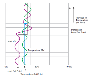Figure 1: Controlled level and temperature using a decoupled control config- uration. MV stands for Manipulated Variable. Taken from [1].

This work is organized as follows. Section 2 describes the multipurpose plant and the supervision module used in this work to implement the MIMO feedback control systems. Section 3 deals with the experimental modelling of the water tank plant. The design and implementation of a MIMO IO as well as a MIMO FO control systems are the topics of Sections

2. Plant Description

Figure 2 shows the multipurpose plant, patented by UTEC (Universidad de Ingenieria y Tecnologia) [6] used in this work, while Figure 3 depicts the corresponding supervision module patented by UTEC [7]. Such equipment is located in the Process Automation Lab of UTEC.

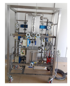Figure 2: The multipurpose plant

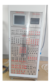Figure 3: The supervision module

Figure 4 depicts the P&ID (Piping and Instrument Diagram) of the multipurpose plant. In Figure 4, T–10 is the water tank plant. Observe that a flow rate q_C of cold water and a flow rate q_H of hot water are entering into T–10. A warm water flow rate q_D is exiting from T–10. Such a tank possesses a water overflow pipe not shown in Figure 4. The on–off valve DV–10 allows the passage of q_C. The control valve FV–10 is used to regulate q_C, while the flow transmitter FT–10 measures q_C.

The hot water flow rate of q_H is regulated by the control valve FV–11 and measured by the flow transmitter FT–11. Inside the tank T–10 there is a temperature transmitter TT–10 and a pressure transmitter PT–10, which is used as a level transmitter. In the tank T–10, there exists an electric heating resistance, whose electric current is controlled by the power controller PW–10 located in the supervision module. Both devices are not used in this paper. This work employs the tank T–20 to produce the required hot water flow rate q_H at a temperature of 50^◦C. The water flow rate q_D exits T–10 through the on–off valve DV–30.

Observe in Figure 4, that the on–off valve DV–20 permits the entering of the flow rate q_C to the tank T–20. This tank possesses a low level swith (LL–20) and a high level switch (HL–20) to indicate if the tank is either empty or filled with water, respectively. The water into the tank T–20 is heated electrically. The temperature into this tank is measured by the temperature transmitter TT–20 and controlled by means of the power controller PW–20 located in the supervision module. A flow rate q_H with a temperature of about 50^◦C is pumped to the tank T–10 by using the pump P–20. The pressure into the pipe that connects tanks T–10 and T–20 is measured by the pressure transmitter PT–20. The speed of the pump is kept constant by means of a speed controller (a variable frequency drive) located in the supervision module.

Figure 4: P&ID of of the multipurpose plant

Figure 3 shows the supervision module that is equipped with breakers, power sources, a PanelView front, two powerful PAC (Programmable Automation Controller), a PLC (Programmable Logic Controller), and a Flex I/O (Input/Output) switch among others. The latter device permits Ethernet communication between the PACs and the PLC of the supervision module with the valves and transmitters of the multipurpose plant. For such a purpose, input and output connectors available on the front panel of the supervisory module (Figure 3) permit to wire the PACs an PLC with the field instrumentation.

The software Studio 5000 from Rockwell Automation is used to elaborate the HMI (Human Machine Interface) and to implement the control algorithms written in structured text language. This work employs the ControlLogic 5000 PAC. Table 1 shows the valued parameters and variables used in this paper.

Table 1: Parameters and variables employed in this work

Symbol	Description	Value
A	Tank rectangular section	0.12 m2
Ao	Output pipe section	5.06×10−4 m2
h¯ = y¯1	Steady state of h	0.2 m
q¯C = u¯1	Steady state of qC	6.66×10−5 m3/s
q¯H = u¯2	Steady state of qH	7.66×10−5 m3/s
q¯D	Steady state of qD	12×10−5 m3/s
g	Earth’s gravity	9.81 m/s2
θC	Temperature of qC	289 K
θH	Temperature of qH	321 K
θ¯ = y¯2	Steady state of θ	304 K
ρC	Water density in qC	998 kg/m3
ρH	Water density in qH	988 kg/m3
ρD	Water density in qD	995 kg/m3
Cp	Heat specific capacity	4186.8 J/(kg–K)
Cd	Discharge coefficient	0.16
α	Discharge factor	3.586 m2.5/s

The outflow rate q_D shown in Table 1 can be computed from

In (1), C_d is the dimensionless discharge coefficient, g is the gravitational acceleration, and D_d is the diameter of the pipe for the outflow q_D. Knowing the steady state values h¯ and q¯_D of h and q_D, respectively,C_d and α can be calculated from

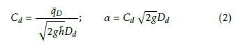Three experiments are performed to determine the discharge coefficient C_d shown in Table 1. For each experiment, the valve FV–10 is opened in a certain percentage to allow the flow rate q_C enter the tank T–10. At the same time, the flow rate q_D is regulated by means of the manual valve until the level h into the tank remains unchanged. At that point, the output flow rate of magnitude q¯_D equals the input flow rate of magnitude q¯_C. Then, the discharge coefficient C_d can be computed from (2). Table 2 shows the results of the experiments. The selected value for C_d is 0.16.

Table 2: Experiment results to obtain Cd

q¯C (m3/s)	h¯ (m)	Cd	α (m2.5/s )
1.45× 10−4	0.162	0.160	3.586
1.95× 10−4	0.307	0.157	3.518
9.72× 10−5	0.092	0.142	3.182

3. Experimental Plant Modelling

Figure 5 depicts the block diagram of the MIMO LTI (Linear Time Invariant) control system, where s is the Laplace operator, G_p(s), G_c(s), G(s), and G_T (s) are transfer matrix functions of the plant, the controller, the open–loop system, and the closed–loop system, respectively. Also, r, e, u, and y are the reference, system error, control, and output vectors, respectively.

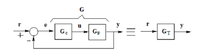Figure 5: Block diagram of the MIMO feedback control system.

From Figure 5: y(s) = G_p(s)u(s), which can be expressed as

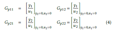
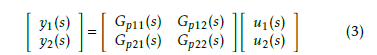The four transfer functions of (3) can be obtained experimentally from

In the figures shown hereinafter, the water level and temperature in the tank are expressed in cm and ^oC, respectively. Let us consider a level transmitter span from 0 cm (0% of the span) to 40 cm (100% of the span). To determine G_p11, the valve FV–10 (Figure 4), which regulates the flow rate of cold water u₁, is opened from 30 to 50%, making y₁ (the water level into the T–10 tank) to change from 10 cm (25% of the span) to 19.5 cm (48.75% of the span) as seen in Figure 6. Using the tangent method in Figure 6, the transfer function G_p11 with gain K_p11 and time constant T_p11 is found to be

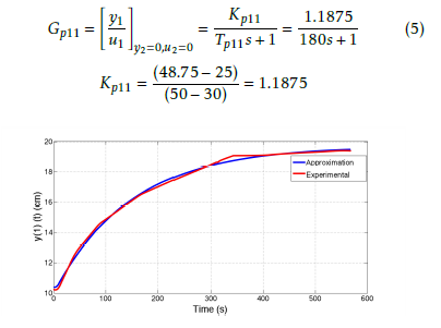Figure 6: Experimental reaction curve for the Gp11 transfer function.

To compute G_p12, the valve FV–11 (Figure 4), which regulates the flow rate of hot water u₂, is opened from 40 to 60%, making y₁ to vary from 10 cm (25% of the span) to 19.5 cm (48.75% of the span) as seen in Figure 7. Using the tangent method in Figure 7, the transfer function G_p12 with gain K_p12 and time constant T_p12 is computed as

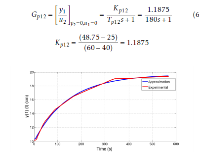Figure 7: Experimental reaction curve for the Gp12 transfer function.

Now, let us consider a temperature transmitter span from

16 ^oC (0% of the span) to 50 ^oC (100% of the span). To find G_p21, the valve FV–10, which regulates the flow rate of cold water u₁ is opened from 30 to 50%, making to drop the temperature y₂ from 32 ^oC (47% of the temperature span) to 24 ^oC (23.5%) as seen in Figure 8. From such a reaction curve, the transfer function G_p21 with gain K_p21 and time constant T_p21 is calculated as

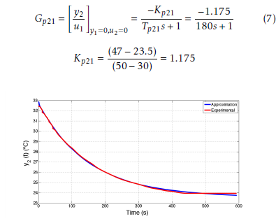Figure 8: Experimental reaction curve for the Gp21 transfer function.

To find G_p22, the valve FV–11 is opened from 40 to 60%, making to change y₂ from 33 ^oC (50% of the span) to 43 (79.4% of the span) as seen in Figure 9. From such a figure, the transfer function G_p22 with gain K_p22 and time constant T_p22 is found to be

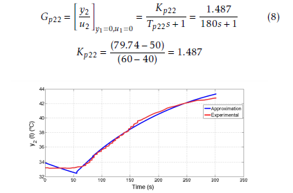Figure 9: Experimental reaction curve for thr Gp22 transfer function.

4. Design of the the Multivariable IO Control System

Consider the following diagonal closed–loop transfer matrix function to assure complete decoupling between the different p inputs.

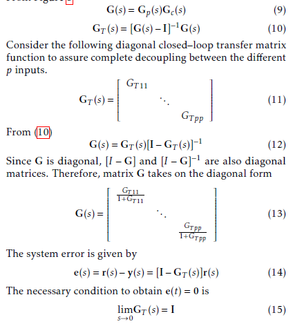For instance, the following G_T (s) transfer matrix meets the condition given by (15)

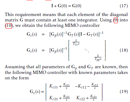Figure 10 depicts the simulation result of the MIMO IO control system using a sampling time of 0.1 s. Reference level and temperature signals were set to 20 cm and 33 ^oC.

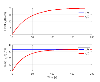Figure 10: Simulated time–responses of the MIMO IO control system. Top graph: controlled level y1(t). Lower graph: controlled temperature y2(t).

Figure 11 depicts the experimental results of the MIMO IO control system employing most of the parameters obtained in the simulation phase. Some parameters required a real– time post–tuning to achieve the desired responses. Observe in Figure 11 that the controlled level y₁(t) possesses a settling time of 225 s, null P.O. (Percent Overshoot), and about a null steady–state error. On the other hand, the controlled temperature y₂(t) shows a settling time of 200 s, a P.O. of 25%, and around a null steady–state error.

It is worth to mention that the MIMO IO controller given by (19) constitutes the structure of the MIMO FO controller to be designed in the next Section.

Figure 11: Experimental time–responses of the MIMO IO control system. Top graph: controlled level y1(t). Lower graph: controlled temperature y2(t).

5. Design of the MIMO FO Control System

The approach used in this section was employed in [9] to control two robot manipulators. The MIMO FO controllers is obtained making fractional the MIMO IO controller given by (19). That is, replacing in (19) all Laplace operators s by s^δ and s^λ, where δ and λ are fractional numbers between 0 and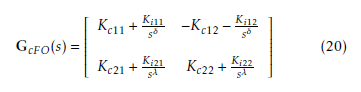

The FO differentiators s^δ and s^λ given in (20) may be approximated by polynomials that depend on the Laplace operator s employing various formulas. For example, for the frequency range of operation [ω_b,ω_h], s^δ and s^λ can be approximated by the following modified Oustaloup filter described in [10]

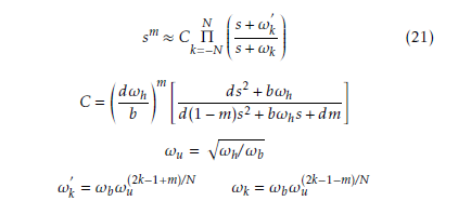According to [10], the Oustalup filter produces a good approximation for b = 10 and d = 9. The frequency range of operation can be obtained from the Bode diagrams of transfer functions of the robot manipulator’s transfer matrix function. However, such an approximation is not employed in this work because we will perform real–time implementation of recursive codes in the discrete–time domain.

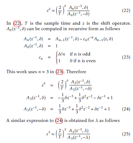
There are various approximations for the FO differentiators s^δ and s^λ as a function of the shift operator z. This work employs the Muir’s recursion method [11], which establishes

Using (20), we formulate u = G_cFOe. Hence, the control laws u₁ and u₂ are formulated as

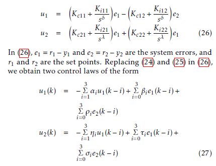In (27), k is the discrete time. Note that parameters α_i, β_i, and ρ_i depend on δ, while parameters η_i, τ_i, and σ_i depend on λ. Recall that fractional numbers δ and λ depend on the sampling time T .

Figure 12 depicts the simulation result of the MIMO FO control system obtained with the following parameters: T₁₁ = 30, T₂₂ = 40, K_c11 = 1.012, K_i11 = 0.005, K_c12 = − 2.334, K_i12 = − 0.013, K_c21 = 0.0846, K_i21 = 0.007, K_c22 = 2.334, K_i22 = 0.013. Reference level and temperature signals were set to 20 cm and 33 ^oC. The simulation phase employed a sampling time of 0.1 s.

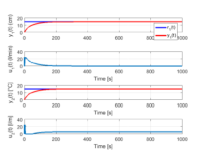Figure 12: Simulation time–responses of the MIMO FO control system. Top graph: controlled level y1(t), second graph from the top: control force u1(t), third graph from the top: controlled temperature y2(t). Bottom graph: control force u2(t).

Figure 13 illustrates the experimental results of the MIMO FO control system using most of the parameters employed in the simulation phase. Some parameters needed a post-tuning to achieve the desired responses. Note in Figure 13 that the controlled level depicts a settling time of 70 s, null P.O., and null steady–state error. Also, the controlled temperature possesses a settling time of 125 s, null P.O., and null steady–state error.

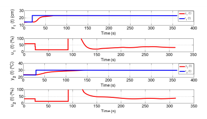Figure 13: Experimental time–responses of the MIMO FO control system. Top graph: controlled level y1(t), second graph from the top: control force u1(t), third graph from the top: controlled temperature y2(t). Bottom graph: control force u2(t).

6. Concluding Remarks

A MIMO IO as well as a MIMO FO control systems were implemented for comparison purposes in this work. At the present, no work that employs a MIMO fractional order controller has been published.

Experimental results demonstrate that the MIMO FO control system performs better because the settling time of the controlled level decreases from 225 s (Figure 11, top graph) to 70 s (Figure 13, top graph), while the settling time of the controlled temperature diminish from 200 s (Figure 11, lower graph) to 130 s (Figure 13, lower graph).

No P.O. (Percent Overshoot) shows the controlled level and temperature using a MIMO FO controller as seen in Figure 13. However, the controlled temperature using a MIMO IO controller depicts a P.O. of 20% as illustrated in the lower graph of Figure 11.

The main problem faced with the employed water tank plant was the supply of hot water in sufficient quantity to perform the experiments.

The simulation of the MIMO IO control systems is necessary to analyse the behaviour of the controlled plant and estimate the tuning parameters required for real–time implementation.

As seen in Figures 11 and 13, the controlled level and temperature do not present oscillations. However, using the decoupled control configuration developed in [1], the controlled level and temperature depicted in Figure 1 show strong oscillations.

Conflict of Interest

The authors declare no conflict of interest.

Acknowledgment

We are very grateful to the Electronic Engineering Department of the Universidad de Ingenieria y Tecnologia (UTEC) for supporting this research work.

1.  TE37 Equipement Control and Instrumentation Study Station, User Guide, Tecquipment Ltd, UK, 2009.
2.  V. Tzouanas, “Temperature and Level Control of a Multivariable Wa- ter Tank Process”, in 120th ASEE Annual Conference & Exposition, Atlanta, Georgia, Jun 23–26, 2013, pp. 1–11.
3.  E. Cornieles, et al., “Modelling and Simulation of a Multivariable Pro- cess Control”, in IEEE ISIE, Montreal, Quebec, Canada, July 9–12, 2006, pp. 1–11. DOI: 10.1109/ISIE.2006.296039
4.  A Rojas–Moreno and A. Parra–Quispe, “Design and Implementation of a Water Tank Control System using a Multivariable PID Controller”, in 6th International Conference on Computing, Communications and Con- trol Technologies (CCCT), Orlando, USA, June 2008. ISBN: 1934272442 9781934272442, Number OCLC: 552110236
5. C. Dinakaran, “Temperature and Water Level Control in Boiler by us- ing Fuzzy Logic Controller”, International Journal of Electrical Power System and Technology, Vol. 1: Issue 1, pp. 27–37, 2015
6.  A. Rojas–Moreno, et al.,“Planta industrial multipropo´sito para control e instrumentacio´n.” Resolution N° 001545–2019/DIN-INDECOPI, May 20, 2019, Lima, Peru
7. A. Rojas–Moreno, et al., “Planta industrial multipropo´sito para control y supervisio´n.” Resolution N° 001035–2019/DIN-INDECOPI, March 28, 2019, Lima, Peru.
8. A. Rojas–Moreno and J. Hernandez–Garagatti, “Modelling of a Multipurpose Water Tank Plant”, in IEEE XXIV International Conference on Electronics, Electrical Engineering and Comput- ing (INTERCON), Cusco, Peru, Aug. 15–18, 2017, pp. 1–4. https://doi.org/10.1109/intercon.2017.8079668
9. A. Rojas–Moreno, “An Approach to Design MIMO FO Con- trollers for Unstable Nonlinear Plants,” IEEE/CAA Journal of Automatica Sinica, vol. 3, no. 3, July 2016, pp. 338–344. https://doi.org/10.1109/jas.2016.7508810
10. C. A. Monje et al., “Implementation of Fractional Order Controllers,” in Fractional–Order Systems and Control. Fundamentals and Applica- tions, Springer–Verlag London Limited 2010, pp. 195–196.
11.  B. Vinagre, et al., “Two direct Tustin discretization methods for fractional-order differentiator/integrator,”
    J. of the Franklin Institute, 340, pp. 349–362, 2003.1016/j.jfranklin.2003.08.001

(Click Here)

(Click Here)