1. Introduction

Human features which are once a very selective parameter has been widely applied as the main input for various research of vision. Detection and tracking of human features can improve the performance of system specifically such as security, safety and also human monitory. For eye tracking system, accurate detection of eyes feature extraction is important as it is the first information eye data and calibration process have to be done. Calibration is the process of measuring the eye gaze point calculation which recording the user’s gaze before an eye tracking recording is started. For the calibration procedure to be achieve in good accuracy, good eye tracking method has to be applied. There are several types of the eye tracking such as electrography, scleral coil and the most popular method of video tracking. This paper is an extension of work originally presented in 2018 International Symposium on Agent, Multi-Agent Systems and Robotics (ISAMSR) conference [1].

Electrography is a method that uses electric potentials measured with electrodes placed around the eyes. N. Steinhausen, R. Prance, and H. Prance [2] applied three sensors of electrodes, P. Aqueveque and E. J. Pino [3] aims on developed a low cost electrography system while H. Manabe, M. Fukumoto, and T. Yagi [4] went into automatic drift calibration for electrography. This method requires only very low computational power but relatively poor gaze direction accuracy to locate where a subject is looking compared to a video tracking even though the time of eye movements can be determined.

For video-based eye tracking, calibration has been created by different approaches and presentations. There is an approach of calibration procedure where the user’s gaze is being calculated and also an approach of calibration-free where the aims are towards removing the calibration process for a fully automatic system.

1. Model and M. Eizenman [5] proposed general method by extending the tracking range for the remote eye gaze tracking system. By using a stereo pair of cameras, the overlapping field of view is used to estimate the user eye parameters. While, J. Chen and Q. Ji [6] proposed general method by gaze estimation without personal calibration which is the 3D gaze estimation. There is also other research such as [7-9] that also applying the same concept of calibration-free and needed more added inputs while adjusting certain parameters. These research shows that calibration-free system is achievable but the need of calibration for measuring accuracy of user’s gaze is still considered as the most important process that cannot be remove in eye tracking.

This paper aims to implement calibration process in order to achieve good accuracy and performance. In order to achieve these objectives, regression technique with good training function is needed. A research from K. Harezlak, P. Kasprowski, and M. Stasch [10] have focus on the process of calibration and analyses the possible steps with ways to simplify this process. The authors compared three regression methods of Classic Polynomial, Artificial Neural Networks (ANN) and Support Vector Regression (SVR) to build the calibration models with presents different sets of calibration points.

      Another approach used detection of the user attention by moving calibration target. This technique is presented by K. Pfeuffer, M. Vidal, J. Turner,A. Bulling and H.Gellersen [11] where the work is focused on smooth pursuit eye movement. This system collects sample of gaze points by displaying a smooth moving target to the user. Three realistic applications have been designed with different abilities in each such as Automated Teller Machine (ATM), stargazing and lastly is the waiting screen application. However, this study showed that too slow and too quick effects the accuracy of the system.

      Facial region is divided into several features such as eyes including pupil, iris, eye corners, eyelid, nose and mouth. There is a method using template matching in facial image presents by Bhoi, N, & Mohanty, M. N. [12] which use the correlation of the eye template as the eye region and P. Viola and M. Jones [13] that used integral images from Haar Basic filters with Adaboost algorithm to create the region of interest around the area of face features.

After taking consideration of eye tracking types and regression method, this paper adapts the same methodology of [10] in building the calibration models with displaying set of calibration points by using video-based tracking and applied Neural Networks algorithm as the regression method with implementation of Viola-Jones algorithm as the eye feature extraction technique. The extracted eye feature information from Viola-Jones become the input data for training the calibration model. To achieve best training model, three training functions are compared for its performance and processing time.

2. Proposed Method

2.1. Displaying the calibration point as a dot

At the beginning of calibration process, stimuli of calibration point must be display to the user. Thus, we have set up two different calibration points, 4 points and 9 points calibration dots each locate at different position. This process is projected to the computer screen in front of the user to generate the raw data of eye detection. The size of the computer screen is 1920×1080 in pixels. The displayed stimuli are divided evenly on the screen as in Figure 1 and 2.

Figure 1: Screen display of 4 calibration points

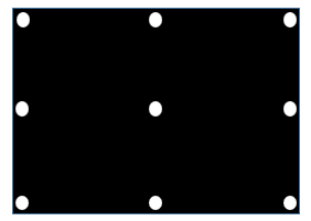Figure 2: Screen display of 9 calibration points

From Figure 1 and Figure 2, the calibration points are being displayed to the user, one by one point. This process is being conducted by using a Logitech HD Pro Webcam C920 which is a full 1080p high definition. This webcam is equipped with the application of video, and photo capture, face tracking, and motion detection with the size of 640×480 in pixels. The setup of tracking the user’s eye features and coordinates are as shown in Figure 3.

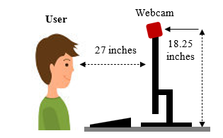Figure 3: Setup of eye tracking

As seen in the figure above, the user’s eye position is being recorded by the web camera. User looked at each point displayed for every 3 seconds at different locations of the calibration point that has been setup. The recorded process is saved in a video format. Thus, the images of user’s interaction must be extracted frame-by-frame before the face and eye features detection being carried out. Figure 4 below shown the image of the user looking towards the displayed stimuli of calibration points of 4 points and 9 points on the computer screen.

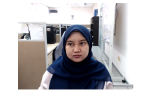Figure 4: Image of user looking towards computer screen

2.2. Face and eye features detection

A video recording is the first step on capturing the user’s eye images for the extraction of the eye center coordinates. As the next step of this research, the face and eye features detection are carried out by using a technique proposed by P. Viola and M. Jones [13], Viola-Jones algorithm. The input data for this algorithm is the image of the user as in Figure 4, that has been extracted frame-by-frame previously. Viola-Jones algorithm is widely known for its ability and performance in detecting the face feature.

6. Viola and M. Jones [13] proposed this method together by using the three main key attributions of integral images, AdaBoost classifier with more complex classifier in a cascade that has been proven to lessen the computational time with high level of detection accuracy. As per mentioned, this research has applied this algorithm which used the Haar-based features that involved the sums of image pixels within the face region in the rectangular areas as shown in Figure 5 and 6.

Figure 5: Face feature detection by Haar-like feature

From Figure 6, it shows the rectangular subset of the detection window that will determines whether it looks like a face.  Two-rectangle features are shown in (A) and (B) while three-rectangle feature in (C) and (D) a four-rectangle feature. Two-rectangular feature is the different between the sum of pixels within two rectangular regions and both have the same size and shape with horizontally or vertically adjacent. As for three-rectangular feature is the different of the sum within two outside rectangles subtracted from the sum in a center rectangle. While the four-rectangle feature is the difference between the diagonal pairs of rectangles.

Figure 6: Example rectangle features shown relative to the enclosing detection window

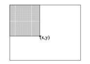Figure 7: The value of integral image at point (x, y) is the sum of all the pixels above and to the left

Integral image is defined as the summation of all pixels in the image at point (x, y) above and to the left.

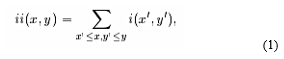where ii (x, y) is the integral image and i (x, y) is the original image (Figure 7). By using pair of recurrences:

where s (x, y) is the cumulative row sum, s (x, -1) = 0, and ii (-1, y) = 0, the integral image can be computed in one pass over the original image. By using integral image, any rectangular sum can be calculated in four array references as in Figure 8.

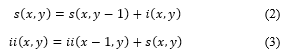
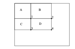Figure 8: The sum of pixels within rectangle D can be calculate with four array references. The value of integral image at location 1 is the sum of pixels in rectangle A. The value at location 2 is A + B, at location 3 is A + C, and at location 4 is A + B + C + D. The sum within D can be computed as 4 + 1 – (2 + 3)

Haar feature used the image integral area to compute the value of a feature and its classifier multiply the weight of each rectangle by its area and the results are added together. Since the detection moved across the image of integral, face recognition filter is applied and when the filter gives a positive answer, it will return feedback as face detected in the current rectangle window.

Each face recognition filter contains a set of cascade-connected classifiers that looks at a rectangular subset of the detection window and determines if it looks like a face feature. The classifier will move to the next classifier until all classifiers and filter give a positive answer, the face feature is considered recognized. The Adaboost algorithm is applied to the training of the cascade classifier to minimize the computational time.

 The process of feature extraction is continued by filter out the eye pair feature. After the eye pair is detected, the algorithm extracted only half of the eye pair from the user’s face feature image. The image of the eye feature is shown in Figure 9 below.

Figure 9: Eye pair feature

 From the half of the eye pair feature, a circle detection algorithm is applied to extract the eye center coordinates. This circle detection is a feature extraction technique for detecting circles called Circle Hough Transform (CHT) where the parameters are containing the center of the circle and the radius. A circle can be described by:

                           (x – a)² + (y – b)² = r²                                  (4)

where (a, b) is the center of the circle, and r is the radius.

 The coordinates will be used as the input data for training the calibration model. When the circle feature has been detected only then the eye center coordinates can be extracted and stored as the raw eye data. Figure 10 shown a circle that are being highlighted in the eye feature image.

Figure 10: Circle detection on eye feature

2.3. Training the calibration model

After all processes of feature extraction has been done, the raw of eye center coordinates have been produced. These data must be normalized before training the data since the size of the user’s eye feature images extracted from the video and the computer screen are different in value.

The normalized eye center coordinates data is stored and be used by Neural Network algorithm for training the model. Neural network can learn and identify images that have been manually trained or labeled for the system to process. A few researches have been conducted using the neural network like [14,15] where they both used neural network for training and identify the parameters of calibration, and input images. Thus, this paper used the approach of neural network to train the calibration model by using the normalized eye center coordinates data from previous process.

There are two sets of calibration points which are 4 points and 9 points that have been distributed at each specific location on the display screen. Thus, two neural networks are been trained for this paper. The type of neural network used is feed-forward back propagation algorithm.

Feed-forward is known for its simplicity of single layer perceptron network which consist of single layer of output nodes where the inputs are fed directly to the outputs via a series of weights. Back propagation is applied with the feed-forward neural network as it is a renowned representative from all iterative gradient descent algorithms that used for supervised learning. This method helps to calculate the gradient descent to looks for the minimum value of the error function in weight space as in Figure 11.

Figure 11: Neural Network architecture with back propagation

As shown in Figure 11, the input given is modeled by using real weights that are usually randomly selected. The output is computed for every neuron from the input layer, to the hidden layer, and to the outer layer. Error is then computed in the output by calculated the differences of the actual output with the desired output. This value will travel back from the output layer to the hidden layer to adjust the weights such that the error is decreased. This process is repeated until the desired output is achieved.

As for the training function, this paper compared the performance and computational time between 3 types of function which are Levenberg-Marquardt known for its fastest, Bayesian Regularization for its efficiency in difficult, small, or noisy datasets, and Scale Conjugate Gradient that requires less memory.

Levenberg-Marquardt (LM) is widely used optimization algorithm for it is outperform simple gradient descent and other conjugate methods. This algorithm provides the nonlinear least squares minimization. Basically, it consists in solving the equation:

                               (J^tJ + ll) d = J^tE                                    (5)

where J is the Jacobian matrix for the system, l is the Levenberg’s damping factor, d is the weight update vector that we want to find, and E is the error vector contained the output errors for each input vector used for training the network. The Levenberg-Marquardt is very sensitive to the initial network weights and does not consider outliers in the data that can lead to overfitting noise. For this situation, we will compare the performance with another technique known as Bayesian Regularization.

Bayesian Regularization can overcome the problem in interpolating noisy data which allows it to estimate the effective number of parameters that actually used by the model such as the number of network weights. It expands the cost function to search for minimal error while using the minimal weights. This function works by introducing two Bayesian hyperparameters, alpha and beta, to tell which way the learning process must seek. The cost function is as follows:

where E_d is the sum of squared error, and E_w is the sum of squared weights. By using Bayesian Regularization, cross validation can be avoided and can reduce the need for testing different number of hidden neurons. However, this technique may be failed to produce robust iterates if there is not much of a training data.

As for Scale Conjugate Gradient, developed by Moller [16], was designed to avoid time-consuming line search. The basic of this algorithm is to combine the model-trust region approach used in Levenberg-Marquardt with the conjugate gradient approach. It requires the network response to all training inputs to be compute several times for each search.

For achieving fast and efficient training model for calibration process, the best training function has to be selected. Thus, the three training functions consists of Levenberg-Marquardt, Bayesian Regularization, and Scale Conjugate Gradient are computed and analyzed the total iterations it takes for achieved minimal error, the processing time and the performance of the algorithm.

The training of 4 points calibration is being carried out first with the total number of neurons for hidden layer of 10, the input data of 200 and the output layer is 150. For each point of the input data, 50 values have been selected. The comparison of those 3 functions are as Table 1 below.

Table 1: Comparison of three training function for 4 points

Training Function	Iterations	Time	Performance
Levenberg-Marquardt	20 Epochs	1m 47sec	1.88e-09 mse
Bayesian Regularization	37 Epochs	5m 29sec	5.39e-08 mse
Scale Conjugate Gradient	76 Epochs	0sec	6.69e-07 mse

From Table 1, Levenberg-Marquardt achieved the minimal training with only 20 epochs of iterations, following with Bayesian Regularization of 37 epochs and lastly with the highest number of iterations of 76 epochs, Scale Conjugate Gradient. For the fastest function, Scale Conjugate Gradient achieved the best computational time with 0 seconds following with Levenberg-Marquardt and Bayesian Regularization. As for the best performance, Levenberg-Marquardt achieved it with only 1.88e-09 mean squared error that is nearest to zero values.

Figure 12: Performance of Levenberg-Marquardt for 4 points calibration model

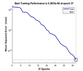Figure 13: Performance of Bayesian Regularization for 4 points calibration model

From Figure 12,13 and 14, it is shown that the best training performance are from the training function of Levenberg-Marquardt, followed by Bayesian Regularization and Scale Conjugate Gradient. As for the regression values which measure the correlation between outputs and targets data, all three training functions achieved a close relationship with R value of 1 as shown in Figure 15.

Figure 14: Performance of Scale Conjugate Gradient for 4 points calibration model

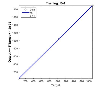Figure 15: Regression values of all three-training function for 4 points calibration

For the training of 9 points calibration, the total number of neurons for hidden layer is 10, the input data of 455 and the output layer is 404. The total number of input data for each point are also 50 values which make the input data for neural network of 9 points calibration is 455. Table 2 shown the comparison of the three-training function for 9 points calibration.

Table 2: Comparison of three training function for 9 points

Training Function	Iterations	Time	Performance
Levenberg-Marquardt	20 Epochs	24m 55sec	1.97e-09 mse
Bayesian Regularization	43 Epochs	1h 25m 44sec	3.56e-08 mse
Scale Conjugate Gradient	446 Epochs	2sec	8.41e-07 mse

From Table 2, Levenberg-Marquardt achieved the minimum iterations of 20 compared to Scale Conjugate Gradient which achieved the highest iteration of 446 epochs. Even though Levenberg-Marquardt achieved the minimum iterations, it cannot be compared with Scale Conjugate Gradient for its computational time. This function required only 2 seconds to finish compared with the other two functions of Levenberg-Marquardt and Bayesian Regularization each takes around 24 minutes and 1 hour 25 minutes.

Since this modeling is from 9 points calibration which contains 455 inputs data, it’s proven that Scale Conjugate Gradient are the fastest training function even by given many datasets. For the best performance of the training model, Levenberg-Marquardt outdone the other two functions by achieved mean squared error of 1.97e-09 as shown in Figure 16 below.

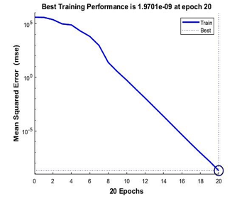Figure 16: Performance of Levenberg-Marquardt for 9 points calibration model

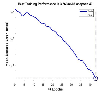Figure 17: Performance of Bayesian Regularization for 9 points calibration model

Figure 17 and 18 are the performance achieved by Bayesian Regularization and Scale Conjugate Gradient for the 9 points calibration model. Bayesian Regularization achieved its best performance of 3.568-08 mse at the iterations of 43 while Scale Conjugate Gradient achieved its performance at 8.41e-07 mse at the iterations of 446.

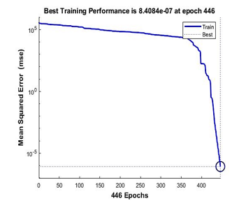Figure 18: Performance of Scale Conjugate Gradient for 9 points calibration model

Figure 19: Regression values of all three-training function for 9 points calibration

      As for the regression values, all the training functions have gained close relationship with R value of 1 as shown in Figure 19.

3. Discussion

The raw eye center coordinates data required normalization which are crucial process that can affect the performance of the data itself. Thus, this normalization can be improved or automated directly in the algorithm so that the process of the training data can be simplified. As for training models, back propagation is proven to be fast, simple and does not need any special mention of the features of the function to be learned but can be quite sensitive to noisy data and the actual performance dependent on the input data given. From the training functions that we have used, taken from the results of their performance, the best training function is Levenberg-Marquardt that is proven the best for its efficiency and good performance while gaining minimum iterations of error with fast computational time even though Scale Conjugate Gradient is a lot faster, the iterations of the error is too high.

4. Conclusions

In this paper, the eye feature extraction and calibration model were conducted by applying Viola-Jones and Neural Network algorithms. Viola-Jones approach using the Haar-like features that involve sums of pixels with integral image by minimizing computational time with Adaboost algorithm and detected the feature of face. As for the Neural Network, the feed-forward back propagation algorithm is applied together and compared the performance and efficiency of three training functions; Levenberg-Marquardt, Bayesian Regularization, and Scale Conjugate Gradient. The overall result shown that these algorithms can be applied and improve the performance and lessen the computational time for eye data training for calibration model.

Conflict of Interest

The authors declare no conflict of interest.

1.  F. N. Ibrahim, Z. M. Zin and N. Ibrahim, “Eye Center Detection Using Combined Viola-Jones and Neural Network Algorithms,” 2018 International Symposium on Agent, Multi-Agent Systems and Robotics (ISAMSR), Putrajaya, 2018, pp. 1-6. doi: 10.1109/ISAMSR.2018.8540543.
2.  N. Steinhausen, R. Prance, and H. Prance, “A three sensor eye tracking system based on electrooculography,” IEEE SENSORS 2014 Proc., pp. 1084–1087, 2014.
3.  P. Aqueveque and E. J. Pino, “Eye-Tracking Capabilities of Low-Cost EOG System,” 36th Annu. Int. Conf. IEEE Eng. Med. Biol. Soc., pp. 610– 613, 2014.
4. H. Manabe, M. Fukumoto, and T. Yagi, “Automatic drift calibration for EOG-based gaze input interface,” Proc. Annu. Int. Conf. IEEE Eng. Med. Biol. Soc. EMBS, pp. 53–56, 2013.
5. D. Model and M. Eizenman, “User-calibration-free remote eye-gaze tracking system with extended tracking range,” Can. Conf. Electr. Comput. Eng., pp. 001268–001271, 2011.
6. J. Chen and Q. Ji, “Probabilistic gaze estimation without active personal calibration,” Proc. IEEE Comput. Soc. Conf. Comput. Vis. Pattern Recognit., pp. 609–616, 2011.
7.  Y. Sugano, Y. Matsushita, and Y. Sato, “Calibration-free gaze sensing using saliency maps,” Proc. IEEE Comput. Soc. Conf. Comput. Vis. Pattern Recognit., pp. 2667–2674, 2010.
8. F. Alnajar, T. Gevers, R. Valenti, and S. Ghebreab, “Calibration-Free Gaze Estimation Using Human Gaze Patterns,” 2013 IEEE Int. Conf. Comput. Vis., pp. 137–144, 2013.
9. Y. Zhang, A. Bulling, and H. Gellersen, “Pupil-canthi-ratio: a calibration- free method for tracking horizontal gaze direction,” Proc. AVI, pp. 129– 132, 2014.
10.  K. Harezlak, P. Kasprowski, and M. Stasch, “Towards accurate eye tracker calibration – methods and procedures,” Procedia – Procedia Comput. Sci., vol. 35, pp. 1073–1081, 2014.
11. K. Pfeuffer, M. Vidal, and J. Turner, “Pursuit calibration: making gaze calibration less tedious and more flexible,” Proc. 26th …, pp. 261–269, 2013.
12. Bhoi, N., & Mohanty, M. N.,”Template Matching based Eye Detection in Facial Image,” International Journal of Computer Applications,12(5), pp. 15-18, 2010 doi:10.5120/1676-2262.
13. P. Viola and M. Jones, “Rapid object detection using a boosted cascade of simple features,” Proceedings of the 2001 IEEE Computer Society Conference on Computer Vision and Pattern Recognition. CVPR 2001, Kauai, HI, USA, 2001, pp. I-I.doi: 10.1109/CVPR.2001.990517
14. M. Wang, Y. Maeda, K. Naruki, and Y. Takahashi, “Attention prediction system based on eye tracking and saliency map by fuzzy neural network,” 2014 Jt. 7th Int. Conf. Soft Comput. Intell. Syst. 15th Int. Symp. Adv. Intell. Syst., pp. 339–342, 2014.
15. E. Demjén, V. Aboši, and Z. Tomori, “Eye tracking using artificial neural networks for human computer interaction.,” Physiol. Res., vol. 60, no. 5, pp. 841–4, 2011.
16. Møller, M. F., “A scaled conjugate gradient algorithm for fast supervised learning,” Neural Networks, 6(4), pp. 525-533, 1993 doi:10.1016/s0893-6080(05)80056-5.

(Click Here)

(Click Here)