1. Introduction

The world is embracing the Fourth Industrial Revolution (IR4.0), driven by nine pillars of technological advancement. They are; Autonomous Robot, Simulation, Horizontal and Vertical System Integration, The Industrial Internet of Things, Cybersecurity, The Cloud Computing, Additive Manufacturing, Augmented Reality, and Big Data and Analytics [1]. As one of the critical elements in IR4.0, robots have been widely used in various areas such as manufacturing, agriculture, retail, and services [2]. To date, there are 1.1 million working robots, and machines worldwide and 80% of the work in the manufacturing of a car is done by machines [3].

In Malaysia, technical and skill oriented educational institutions are one of the critical feeders for skilled and knowledgeable human capital in the area of robotics. The country has realized the importance of technical and vocational education and training (TVET) in spearheading the country’s excellence in economic and technological development [4]. Thus, it is essential to engage students in this field further by creating new, affordable robotics platforms through which they can involve themselves in current technologies at a fraction of the cost.

Most industrial robotics producers such as ABB, KUKA, MOTOMAN, and FANUC do provide robotic educational packages based on their smallest robot available. Nonetheless, due to their rigid structure, strict safety measures need to adhere to [5]. This will incur additional costs to the institution. Therefore, a small-scaled six-axis robot is seen as suitable for use in an educational setting. The robot system requires less damage and is safer when in contact with a human because it will generate less momentum when in motion compared to the metal structure.

One of the available techniques to construct a mechanical structure of a robotic arm manipulator is by using Fused Deposition Modelling (FDM). With this method, a polymer-based filament such as acrylonitrile butadiene styrene (ABS), Polylactic acid (PLA) or nylon is extruded in semi-liquid form through a heating process and deposited layer by layer until a 3D object is formed. It provides a trade-off between strength and cost. This is vital in a lightweight robot configuration. Its ease of use and fast time from design to manufacturing also makes FDM printers prevalent in small manufacturing enterprises, design offices, and private residential [6, 7].

This study aims to design and develop a six-axis robot manipulator using FDM for educational purpose typically for TVET schools. This robot is small and compact compared to its vast industrial counterparts. Besides training, this robot can also be advertised to small and medium businesses who seek to increase their productivity through automation.

2. Methods

The methodology begins with studying existing designs of robot manipulators with the same payload and using open-access assembly drawing of a desktop-size robot by Chris-Annin [8], which is known as the AR2. Using SolidWorks 2018, a model was redrawn. This process considers the actuator sizing, the mechanism such as the belts, the gears, and the type of material for printing.

The tooth-belt transmission mechanism was selected for joint-1 to joint-5 because it is simple to integrate into CAD design. Joint 6 has the tool with a direct connection to the actuator. The drawings were fed to the FDM machine to produce the mechanical structure. All the joints apply the stepper motor with an encoder as the actuator. The controls would employ step input, and the encoder functions for feedback. The ABS was selected as it is a rigid material for a sturdy structure to mount the stepper motors. ABS is cost effective as compared to nylon and carbon fiber.

2.1. Classical Denevit-Hartenberg Representation

Before production, the CAD design requires parameter validation. As a start, the arm parameters have to be defined and later analyzed according to the standard Denevit-Hartenberg (stdDH) convention. Table 1 list the proposed AR2 arm parameter [9]. Each of the parameters determines the arm configuration and its outlook. Therefore, solid modeling using CAD is possible.

Table 1: The arm parameter for AR2. The d and the α parameters govern the arm’s size.

Joint №			(mm)	(mm)
1		-90	169.77	64.20
2		0°	0	30.50
3		90°	0	0
4		-90°	-222.63	0
5		90°	0	0
6		0°	-36.25	0

The kinematic chain seen in Figure 2 is built conforming with the stdDH. The orientation of the joint frame is significant because it allows the designer to decide how to assemble the actuator. It is usually that the actuator is attached along the z-axis. Using the tools found in the Robotic Toolbox module, the information is realized in the form seen in Figure 1.

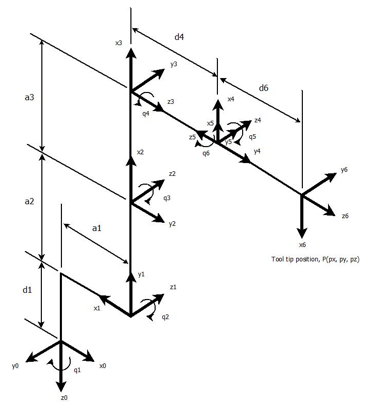Figure 1: The kinematic chain that represents AR2. The configuration is unique. A correct configuration provides the descriptions that permit the designer to test for arm position and motion. If the setting is wrong, then the results from the analysis will be incorrect. By itself, the developed robot will not function as desired.

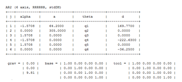Figure 2: The simulated arm parameter runs onto Scilab. The outcome is the reproduction of the arm parameter seen in Table 1. Having the arm parameter configured correctly, the tools in Scilab let the robot to be evaluated with convincing results. The ‘6-axis’ means that the robot has six joint where an actuator drives each joint, the ‘RRRRRR’ represent a revolute type of all the joint, the ‘stdDH’ depicts that the robot is specified according to the standard Denevit-Hartenberg convention.

2.2. Forward and Inverse Kinematics

Given the pose, and by analyzing the mechanisms, the relationship between the locations concerning the base, the serial chain can be derived. The device is dependent on the method of actuation typically for the forward kinematics problems where the tool pose can be found when the values of the joint variables of the actuated joints are given [10]. It is known that the inverse kinematics for the chain can have non-unique solutions, and so does the inverse kinematics.

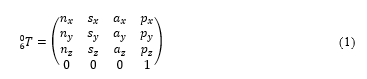
The definition of the forward kinematic is given in (1) [11]. The vector in the last column except the last cell represents the tooltip position. In Figure 1, the said position is charted in frame 6. The remaining columns, up to row 3 define the tool orientation. If the joint angles are stated, then (1) can be evaluated. The results will be the tool’s pose and orientation.

So, to test for the robot’s plot, the joint angles need to be defined. Suppose the arm is positioned to vertical upright, the joint angle vector is then . Figure 3 shows the arm’s position realized through Scilab. At this juncture, the forward kinematics is defined in  (2) that has the tool tip position vector as .

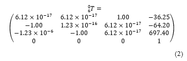
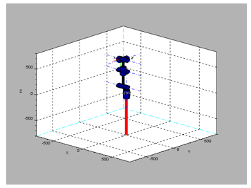Figure 3: The arm is programmed to raise vertical upright. At this posture, the arm is assumed in the home position.

The inverse kinematics, however, does not define in a straight-forward manner as the forward kinematics. A complicated derivation involves in determining each joint position. The general idea behind inverse kinematics is that given the desired tool position, the resulting joint angles may be obtained. Suppose the desired position vector is . Then the respective joint angle may be computed using the available tools in the Robotic Toolbox. The inverse kinematics results the required joint angles as , which exactly computed as the direct kinematics’ inputs.

2.3. Trajectory Planning

The joint space trajectory is based on quintic polynomial with zero boundary condition for velocity and acceleration. The path of each joint has to be planned so that the tooltip position reach a coordinate. For a quintic polynomial, (3a-3c) define the position trajectory, velocity trajectory, and the acceleration trajectory, respectively.

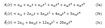In (3a-3c), the constant parameter  is not defined because the automatic derivation is made in the Scilab environment. Every incident of the joint trajectory is unique. It is, therefore, the value for the constant  dependent upon the incident of the joint trajectory as a function of the desired . Because there are six joints, the index . At most, there are six functions for the position trajectory. Similarly, the velocity trajectory and the acceleration will each has six functions, tops. In total, there should be eigtheen plottable functions as long as there is a position change for a joint.

3. Results

3.1. Assessment of Kinematics Solutions

Evaluation for the inverse kinematics solutions was done by assuming some desired positions. The answers were then compared with the inputs fed to the homogeneous transformation matrix defined in  (1). Setting the Robotic Toolbox’s ikine (inverse kinematics) function with pinv (pseudo-inverse), the inverse kinematic solutions are shown in Table 2, especially columns three and four. The respective joint positions were obtained using the desired positions mentioned in the preceding. For the computational purpose, seen in column three, the initial positions were adjusted very close to the earlier forward kinematics’ joint angles.

Table 2: Evaluation of inverse kinematics solutions. Scilab’s ikine function was used because the arm’s wrist is not spherical. The answers were copied from Scilab’s console. The ‘D’ notation is the power of ten.

Forw. kinem. inputs	Position Vector	Initial joint angles	Inv. kinem. solutions	% error
-1.5707963 -1.5707963 -1.5707963 -1.5707963 -1.5707963 -1.5707963	-36.250000 -64,200000 697.40000	-1.4707963 -1.4707963 -1.4707963 -1.4707963 -1.4707963 -1.4707963	-1.5707963 -1.5707963 -1.5707963 -1.5707963 -1.5707963 -1.5707963	0.0000001 0.0000005 -0.0000012 6.542D-08 -0.0000002 0.0000007
-1.0471976 -0.7853982 -0.6283185 -0.5235988 -0.4487990 -0.3926990	280.26218 -466.5156 358.95479	-0.9471976 -0.6853982 -0.5283185 -0.4235988 -0.3487990 -0.2926991	-1.0471976 -0.7853982 -0.6283185 -0.5235988 -0.4487990 -0.3926991	9.235D-09 5.057D-08 -8.476D-08 -8.089D-08 0.0000001 0.0000001
-0.7853982 -0.6283185 -0.5235988 -0.4487990 -0.3926991 -0.3490659	384.6609 -393.17299 256.28879	-0.6853982 -0.5283185 -0.4235988 -0.3487990 -0.2926991 -0.2490659	-0.7853982 -0.6283185 -0.5235988 -0.4487990 -0.3926991 -0.3490658	-7.513D-09 3.196D-08 -0.0000001 -0.0000004 7.452D-08 0.0000004

The first column represents the forward kinematics solutions that yielded the position vectors. Based on the position vectors, the ikine function was executed. In the last column, it was obvious that the percent errors when compared between the forward kinematics inputs and the inverse kinematics solutions were minimal. The overall solutions looked convincing. Therefore, the stdDH model applied was valid.

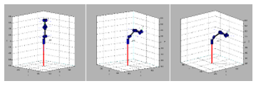Figure 4: The arm’s poses and positions. From left, the start pose and position. The stopover pose and position and lastly, the final pose and position. The snapshots when combined, would reveal a planned trajectory. They were three tool tip’s positions that a straight line path was made possible.

The arm was made to move in the joint space trajectory. The respective joint positions would be determined according to the desired tool tip’s position. A tool tip’s path in the Cartesian space was planned that three positions were defined to complete the track. The position vectors in Table 2 were used as the coordinate of the point in the Cartesian space that the desired positions were  , , and  to achieve a straight line path. The first was the start position, the second was the stopover position, and the last was the final position where Figure 4 describes the incident.

3.2. Assessment of the Trajectory Planning

For the tooltip position that initiated from the start to the second point within five seconds, the results for the joint trajectories are shown in Figure 5. From the left is the position trajectories for all the joints. It follows for the velocity trajectories, and the acceleration trajectories, respectively.

Joint-6 represents the maximum velocity at about 2.5 seconds, the maximum acceleration at about one second and the minimum at about 4.0 seconds. Joint-1, however, makes the least positions, velocities, and accelerations. Similarly, Figure 6 exhibits the motion trajectories within 2.5 seconds, which is a one-half time range from the previous. The results show comparable patterns from the former. With less position change, the velocities and the accelerations were doubled.

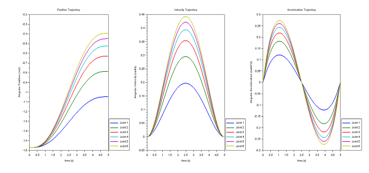Figure 5: The joint trajectories for joint 1 to joint 6 that the tooltip moves from   to . The curves were plotted because all joints experienced a position change. For the position trajectory,  (3a) is the function where the time range was set for 5 seconds. The velocity trajectory was the derivative of the position trajectory,  (3b) is the function. Similarly, the acceleration was the derivative of the velocity trjectory,  (3c) is the function.

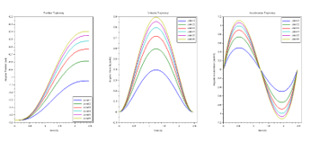Figure 6: The joint trajectories for joint 1 to joint 6 that the tooltip moves from   to .  The time range was set for 2.5 seconds.

For the tooltip position that moved from the second point to the final point within five seconds, the results for the joint trajectories are shown in Figure 7. From the left is the position trajectories for all the joints. It follows for the velocity trajectories, and the acceleration trajectories, respectively. Joint-6 represents the least velocities, accelerations but the most for the position trajectories. In contrary, joint-1 made the least position trajectories but the most for the velocities and accelerations. The results show comparable patterns from the previous. With fewer position change, the velocities and the accelerations were amplified.

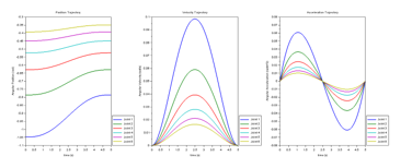Figure 7: The joint trajectories for joint 1 to joint 6 that the tooltip moves from   to . The time range was set at 5 seconds.

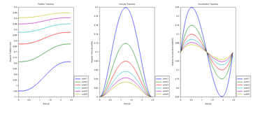Figure 8: The joint trajectories for joint 1 to joint 6 that the tooltip moves from   to . The time range was set at 2.5 seconds.

3.3. Fabrication of the Arm Structure

Figure 9 shows the constructed robot structure. It was produced using ABS filament. Due to the ABS material color, some of the parts are red, while others are white. From computation, it was estimated that the weight of the arm structure alone is 5.5 kg. With the stepper motors weight, the total weight of the manipulator is about 8.4 kg.

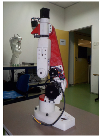Figure 9: The fabricated manipulator is on the foreground. The project is on progress where at this stage, the controller module has not been assembled. As such, there are loose wires and connectors seen on the structure.

4. Conclusions

This paper shows the preliminary design works of a six-axis robotic arm for TVET education purposes. The arm should be capable of lifting load not more than one kilogram. The overall weight of the arm was acceptible for a training type robot and is comparable to others in the market. Before it was constructed, the arm parameters were assessed using Scilab as the tool and the traditional and fundamental methods: the Denevit-Hartenberg representation, the forward kinematics, the inverse kinematics, and the trajectory planning. The outcomes showed that the arm was working well on positioning and path planning. Therefore, the complete assembly of the robot should be able to assume a role in education and training.

Conflict of Interest

The authors declare no conflict of interest.

Acknowledgment

The authors would like to thank Universiti Teknikal Malaysia Melaka for financial support through PJP/2018/FKP (10C)/S01636 research grant, Nick Mathews A. Samuel for the arm fabrication and assembly.

1.  M. Rüßmann, M. Lorenz, P. Gerbert, M. Waldner, J. Justus, P. Engel, et al., “Industry 4.0: The future of productivity and growth in manufacturing industries,” Boston Consulting Group, vol. 9, 2015.
2.  K. Schwab, The fourth industrial revolution: Crown Business, 2017.
3.  W. Knight, “This robot could transform manufacturing,” MIT Technology Review, 2012.
4. M. Sandhya, “TVET to meet industry needs,” in The Star, ed, 2017.
5. V. Gopinath, F. Ore, S. Grahn, and K. Johansen, “Safety-Focussed Design of Collaborative Assembly Station with Large Industrial Robots,” Procedia Manufacturing, vol. 25, pp. 503-510, 2018. https://doi.org/10.1016/j.promfg.2018.06.124.
6. Q. Zhang, G. Sharma, J. P. Wong, A. Y. Davis, M. S. Black, P. Biswas, et al., “Investigating particle emissions and aerosol dynamics from a consumer fused deposition modeling 3D printer with a lognormal moment aerosol model,” Aerosol Science and Technology, pp. 1-13, 2018. https://doi.org/10.1080/02786826.2018.1464115.
7. D. Owen, J. Hickey, A. Cusson, O. I. Ayeni, J. Rhoades, Y. Deng, et al., “3D printing of ceramic components using a customized 3D ceramic printer,” Progress in Additive Manufacturing, pp. 1-7, 2018. https://doi.org/10.1007/s40964-018-0037-3.
8. Chriss-Annin. (2018). AR2. Available: https://github.com/chris-annin/ar2.
9. P. I. Corke, “A simple and systematic approach to assigning Denavit–Hartenberg parameters,” IEEE transactions on robotics, vol. 23, pp. 590-594, 2007.
10. R. C. Gonzalez and R. E. Woods, Digital Image Processing 2nd ed. Upper Saddle River, New York: Prentice Hall Press, 2002.
11. J. J. Craig, Introduction to robotics: mechanics and control vol. 3: Pearson/Prentice Hall Upper Saddle River, NJ, USA:, 2005.

(Click Here)

(Click Here)