1. Introduction

This paper is an extension of work originally presented in OCEANS’18 MTS/IEEE Kobe/Techno-Oceans 2018, May 28-31, Kobe Japan [1].

Typical tsunami warning system includes the following parts: wave generation, propagation over the water area under study, and inundation of a dry land. Aiming to achieve real time tsunami danger prediction, we address the question of fast determination of tsunami source parameters. Having such information, there are several software packages for numerical simulation of wave propagation and inundation mapping. Here we refer the reader to MOST (Method of Splitting Tsunami – official tool of the NOAA UnS tsunami warning centers), see [2-4], and TUNAMI, see [5,6].

In any case numerical simulation of wave propagation requires the initial data, say initial sea bed displacement at tsunami source. In this paper we address the question of rather fast reconstruction of the sea surface displacement at tsunami source. As an input data we use direct measurements of the wave profile (time series), obtained at any sensor system. As is well known, a number of deep-water pressure recorders are located all around Pacific Ocean, they measure and send such data via satellite channels. Among these systems we would like to mention the USA DART (Deep-ocean Assessment and Reporting of Tsunami) buoys (https://nctr.pmel.noaa.gov/Dart/), and DONET (Dense Oceanfloor Network system for Earthquakes and Tsunamis) pressure gauge network system, which is under construction in Japan (https://www.jamstec.go.jp/donet/e/).

Our goal is to recalculate these direct measurements of the water column over a single sensor (which is nothing but a curve of the wave profile) in terms of 2D function of initial sea surface displacement at tsunami source. In general mathematical statement it is not possible to solve this problem. So, we use the so-called “Calculation in Advance” inversion strategy [7].  It has been proposed to cover the subduction zone (area of possible tsunami sources) with the system of 100×50 km rectangles (typical size of the seabed displacement zone for tsunamigenic 7.5 M earthquake). In case of Alaska-Aleutian subduction zone there are 50 of such Unit Sources (UnSs), composed in two alongshore lines. Then a typical (for this region) shape of the initial sea-bed displacement, normalized with an amplitude of 0.57 m, is used at each UnSs as tsunami wave source. Propagation of such wave from all the UnSs were numerically calculated (in advance) over the entire Pacific Ocean according to the approximation of shallow water system. As a result, a database of the calculated tsunami wave profiles, generated by the source of the same initial shape at all UnSs, is available for all grid points of the Pacific Ocean.

Now, having the measured (real) wave profile at certain sensor location, one can approximate this curve with the help of linear combination of calculated wave profiles from a number of UnSs, picking up at the same point of sensor location. In other words, the problem is to determine the amplification coefficients for the UnSs such that the corresponding linear combination of UnSs (say, a Composed Source – CS) provides a good approximation of the initial sea-bed displacement.

The similar approach named SIFT – Short-term Inundation Forecasting for Tsunamis (https://nctr.pmel.noaa.gov/Pdf/SIFT _3_2_2_Overview.pdf) is used by NOAA (USA) for wave height assessment in grid points of computational domain. As well as in the method presented here, on the basis of “computations in advance” of the tsunami height distribution from the set of Unit Sources the authors [7] reconstruct the CS. Unlike the method presented here, by search of set of coefficients in linear combination of UnSs, the SIFT system uses the combinatory search of values of coefficients giving a discrepancy minimum between real and calculated tsunami wave series in several tsunami detectors. Such approach requires a lot of processor time if CS consists from more, than 5 UnSs. There is no such a shortcoming of the approach here proposed, where CS restoration time practically does not depend on quantity of UnSs involved. By the way, authors of this article also took part in development of an algorithm for source inversion in the SIFT forecasting system.

This approach has been many times tested against the field observations after near field and trans-oceanic events. Amazing agreement has been observed by comparison of computed wave, generated by a calculated CS, and measurements taken at various gauge stations. Nowadays, all subduction zones around Pacific, Atlantic, and Indian Oceans were covered with such systems of UnSs unit sources (https://nctr.pmel.noaa.gov/propagation-database.html); synthetic marigrams at every grid point from every source have been saved in a specialized database. One of the problems is to choose the aforementioned amplification coefficients in an automated mode. The orthogonal decomposition approach to handle this was proposed in [8] and then tested in [1,9]. It happens that even a part of the first wave period is enough to determine the CS – the set of amplification coefficients. In this paper we continue to study the problem of robust determination of sea surface displacement at tsunami source by a part of the wave profile.

The paper is arranged as follows. We first describe the proposed orthogonal decomposition algorithm and provide the mathematical ground behind it. In the numerical section we briefly describe digital bathymetry in use and the parameters of realistic CS, which has a feature of the reconstructed source of historical event of 1707 [10]. Then we provide the obtained numerical results in the form of a table. Finally, numerical results are discussed.

2. Orthogonal decomposition algorithm

2.1. Mathematical ground of algorithm

Here we provide the brief explanation of the algorithm for reconstruction of the CS. More detailed description one can find in [8].

Let f(t) be the marigram – time series, obtained at any particular sensor (DART buoy, bottom cable sensor of DONET, or other). We will use notations  for simulated wave profiles, calculated (according to the linear or nonlinear shallow water approximation) at the same point of sensor location, by direct numerical modeling of the tsunami wave propagation. It is understood, that the subindex k refers to a tsunami wave initiated by the normalized sea surface initial profile of a given shape from the k-th UnSs. We assume that all these functions, , are linearly independent. We are looking for coefficients, , for the linear combination of these functions, which provide the best approximation of the function f(t) in  norm:

So, we consider the problem of optimal approximation of a given function, f(t), by the linear combination of the finite subset of functions from the system . Suppose that the system is orthogonal and normalized according to:

Here t₀ stands for the time moment when the wave approaches the closest receiver, T is the time of the latest (of all receivers) full period on marigram which is concerned as the end of the second phase of tsunami. For sensors which are more distant off the coast than a source, the second phase of tsunami is positive, and for those which are closer to the shore, it is negative.

As is well known in the Fourier series theory, the coefficients of such optimal approximation are nothing but the Fourier coefficients of expansion of f(t) in a series with respect to  (see, for example, [11]).

2.2 Algorithm description

Based on the statement above, the following algorithm was proposed in [8] and tested in [1,9] for searching the coefficients of the linear combination allowing optimal approximation of the given function. It includes three steps.

• The calculated set of “marigrams”, , from the unit sources should be orthogonalized and normalized, according to equations (2)-(3).
• The measured marigram, f(t), should be expanded to the Fourier series with respect to obtained orthonormal system of functions.
• The so-determined Fourier coefficients should be recalculated in terms of initial functions .

Let us transform the given system  to the corresponding ortho-normal system,  , with respect to the scalar product (2). Let

Suppose that pairwise orthogonal nontrivial functions  are already constructed. We will look for the function  in the form:

i.e. we obtain the next function, , as the linear combination of the new function,  , and the already constructed ortho-normal ones, . The coefficients, , in formula (5) should be found from the conditions that the new function,  , is orthogonal with all the previous ones, , and normalized. Thus, the coefficients in (5) are calculated according to:

As is well known in calculus, the optimal  approximation, according to criteria (1), of a given function f by the linear combination of orthogonal and normalized functions,

is achieved at the Fourier coefficients,  , of the function f(t), decomposition with respect to the system  :

So, to solve the original problem (1), we only need to provide the coefficients (8) in terms of the original basis functions .

It is just an algebraic exercise to conclude that the desired coefficients, , in expression (1), are calculated through the given coefficients,   from the formula (8), as follows:

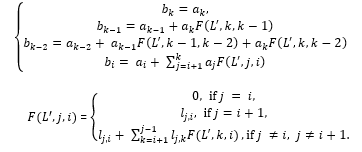So, the proposed algorithm to approximate the given marigram, f(t), by the linear combination of synthetic marigrams, , k=1,…,N, in order to achieve minimal  difference (1), is as follows.

We first transform the system  to the orthogonal system, , and normalize it according to formulae .

Then the recorded marigram, f(t), is decomposed to the part of Fourier series with respect to obtained orthogonal and normalized (see (1), (2)) basis, , by the formula (8).

Finally, the obtained Fourier coefficients, , are recalculated in terms of coefficients, , of the original linear combination (1), by means of (9).

3. Numerical experiments

Numerical experiments were arranged in the area around the south-east coast of Japan (eastern Kyushu, Shikoku islands and Kii peninsula. Geography, bathymetry and location of UnSs and CSs in this region are shown in Figure 1.

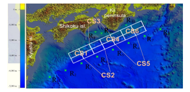Figure 1: Digital bathymetry of the water area under study. White rectangles show positions of model tsunami sources. Green crosses (R1-R8) indicate locations of artificial sensors. Green check marks (R9-R11) show the selected sensors of DONET.

3.1. Digital bathymetry

Numerical experiments were arranged at the gridded bathymetry around Eastern Kyushu, Shikoku Island and Kii Peninsula (southern part of Japan), built on the basis of Japanese bathymetric data produced by the Japan Oceanographic Data Center (JODC), presented in Figure 1. This digital gridded bathymetry has the following characteristics:

Size of array is 3000 x 2496 nodes;

Grid steps are 0.003 and 0.002 degrees (which means 280.6 and 223 meters, respectively);

Domain covers the area approximately between 131° E and 140° E, 30° N and 35° N.

3.2. Composition of tsunami source

In the course of numerical calculations model tsunami sources were formed of UnSs of 100х50 km in size located in two rows along the coast (Figure 1). Each of the six composed sources (CS), having the sizes of 200х100 km, is presented as the linear combination of four UnSs with given amplification coefficients (1.4; 1; 1.5; 1.1). For this set of coefficients, the maximum surface elevation in the source area is equal approximately to 3 m, and minimum water level there is estimated as -1.5 m (Figure 2). Bigger coefficients correspond to UnSs more distantly located off the coast. Numbering of CSs begins with UnSs which are at the western edge the source area (Figure 1). Two of them (the first and the last) are indicated in Figure 1. The ocean bottom displacement in the CS used for computations is shown in Figure 2.

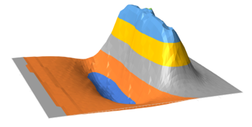Figure 2: Shape of the initial surface displacement at the Composite Source used for numetical experiments.

We assume precision of 10% as the value of reasonable accuracy of the tsunami height estimation. This value allows to determine parameters of the wave near the shore with the same precision, which is enough for the rapid tsunami hazard evaluation. It means that maximum difference between the initial and calculated surface displacement is less than 10 cm for a typical initial displacement height of 1 m. Accordingly, the deviation of 1 m is considered acceptable in case the wave height is 10 m.

As a rule, a part of the wave profile from the beginning to the zero level after the highest amplitude point (see Figure 2) is sufficient to reconstruct the amplification coefficients with a particular precision. So, we tried to determine how smaller could be a part of wave profile to keep the error in reconstructed ISSD amplitude within 0.1 discretization. The location of the model tsunami source centers for numerical calculations are chosen according to estimation of the source of the major tsunami, expected, according to [10], in the near future in the Nankai subduction zone (Figure 3 is taken from [10]). The size of the model sources corresponds to a tsunamigenic earthquake of magnitude 8.0.

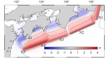Figure 3: The expected distribution of the initial water surface displacement in the tsunami source at the Nankai subduction zone, [10].

3.3. Positions of sources and sensor network

The virtual sensors network consists of one row of virtual deep-water wave detectors, installed along the Nankai Trough (R₁-R₈, indicated by green crosses in Figure 1). In addition, 3 sensors of DONET were also included to observation network system for source restoration in our numerical experiments. These sensors are indicated in Figure 4 as black squares, R₉, R₁₀ and R₁₁. Reconstruction of a source means determination of coefficients in the linear sum of UnSs composing CS.

3.4. Numerical experiments

As a result of numerical experiments, the tsunami wave signal from each of the six locations of CS (see Figure 1) was recorded by 11 detectors, R1-R11, given in Figures 1 and 4. By means of the described method, the minimum length of a wave signal, sufficient for determination of coefficients in the linear sum of UnSs (Necessary Part of Wave Profile – NPWP) have been determined with the required accuracy. These lengths as a percentage to length of the full wave period which means complete first two phases (positive and negative) of a wave are summarized in Table 1. The first column shows receiver’s number (1-11). In the second column one can find the Composed Source number (1-6). In the third and the fourth columns the length in seconds of NPWP and the full wave period are presented, respectively. Column number 5 gives the length of NPWP in percentage of the full tsunami period.  The last two columns present the NPWP ending time instance and the wave arrival time to a shore.

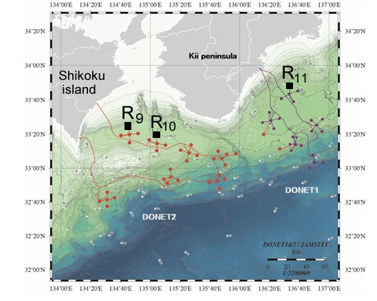Figure 4: Configuration of DONET-1 and DONET-2 system at the south-east of Japan (https://www.jamstec.go.jp/donet/e/). The existing sensors are in violet and sensors under construction are indicated in red. Black squares show three sensors, which positions were used for artificial sensors.

The duration of NPWP counted from the moment of wave arrival at receiver. More important for us is the end of NPWP on the record (column 6 in the Table 1). This record starts simultaneously with the initial ocean surface displacement. It is the same moment as regarded as zero in tsunami travel time. So, if NPWP (on record) is less than the tsunami travel time to the coast, then we have some time for reconstruction of CS and for estimation of the expected wave height near a shore.

Table 1: Numerical tests Parts of the entire wave profile (in percents), enough to determine the source parameters

Receiver	CS	NPWP, sec	Period, sec	NPWP, % of full wave period	Time required for accuracy to be achieved (from the generation moment), sec	Wave arrival time to a shore, sec
1	1	1511	1736	87.0	1511	837
2	1	224	1561	14.3	224	837
3	1	730	2553	28.6	998	837
4	1	442	1422	31.1	1731	837
5	1	419	1262	33.2	2313	837
6	1	1365	1608	84.9	3575	837
7	1	121	3867	3.1	2565	837
8	1	141	2949	4.8	3178	837
9	1	530	1257	42.2	698	837
10	1	496	1260	39.4	519	837
11	1	223	981	22.7	223	837
1	2	409	1311	31.2	409	876
2	2	223	1070	20.8	223	876
3	2	1724	2614	66.0	1724	876
4	2	474	2640	18.0	1327	876
5	2	679	1056	64.3	2057	876
6	2	542	2509	21.6	2469	876
7	2	247	3837	6.4	2369	876
8	2	328	2875	11.4	3040	876
9	2	219	1116	19.6	223	876
10	2	261	1031	25.3	261	876
11	2	293	1080	27.1	293	876
1	3	480	1359	35.3	480	525
2	3	223	1149	19.4	223	525
3	3	2043	2489	82.1	2043	525
4	3	728	1803	40.4	1012	525
5	3	922	1859	49.6	1786	525
6	3	1226	1594	76.9	2617	525
7	3	632	3844	16.4	2450	525
8	3	428	2769	15.5	2827	525
9	3	221	1003	22.0	223	525
10	3	311	904	34.4	311	525
11	3	380	1282	29.6	475	525
1	4	811	1322	61.3	1075	465
2	4	223	1134	19.7	223	465
3	4	419	2479	16,9	419	465
4	4	698	3203	21.8	698	465
5	4	868	1735	50.0	1183	465
6	4	1595	2767	57.6	2489	465
7	4	340	1503	22.6	1776	465
8	4	377	2808	13.4	2483	465
9	4	221	1359	16.3	223	465
10	4	223	1274	17.5	223	465
11	4	503	1482	33.9	928	465
1	5	596	1572	37.9	1405	510
2	5	988	2057	48.0	1090	510
3	5	1442	2585	55.8	1442	510
4	5	1450	1470	98.6	1450	510
5	5	1065	1882	56.6	1065	510
6	5	925	2183	42.4	1215	510
7	5	406	1895	21.4	1411	510
8	5	447	3062	14.6	2080	510
9	5	294	1484	19.8	301	510
10	5	350	1437	24.4	403	510
11	5	598	1746	34.2	1280	510
1	6	515	1138	45.3	1690	630
2	6	735	1201	61.2	1355	630
3	6	825	2457	33.6	1243	630
4	6	223	1497	14.9	223	630
5	6	568	1552	36.6	568	630
6	6	654	2124	30.8	654	630
7	6	630	2226	28.3	1093	630
8	6	460	3260	14.1	1625	630
9	6	389	1418	27.4	662	630
10	6	476	1361	35.0	851	630
11	6	539	1424	37.9	1523	630

Numerical experiments showed that in most cases use of even a wave record only from one sensor allows to restore the source (coefficients in the linear sum of UnSs) with the required accuracy, using only a part of a wave signal (less than a half of its full period). From the results presented in Table 1 it is visible that for each CS there are several sensors, processing of a wave signal from which allows to restore the source with the required accuracy even before arrival of a wave to the nearest coast. In particular, for CS1 those are detectors R1, R2, R9, R10 and R11. For CS2 those will be sensors R1, R2, R3, R9, R10 and R11. And so on.

4. Discussion

The fact that among such sensors there is always a tsunami detector which is included to observation system DONET (Figures 1 and 4) is important. In these sensors (R9-R11) the first phase of tsunami on the wave record is negative (surface inundation), and then the surface elevation is coming. Finally, we can conclude that with the help of observation network described the tsunami warning system is able to estimate expected wave heights along the coast before its arrival there.

By results of the numerical experiments given in table 1 one can notice that the length of NPWP for restoration of some CSs by records of some sensors exceed 80% of the full period of a wave. Though, in most cases duration NPWP does not exceed 50 percent of the tsunami period. In particular, more than 80 percent of the full wave period is required for sufficient-quality restoration of CS having number 1 by means of sensors R1 and R6. The CS3 by means of sensors R3 and R6. And, at last, CS5 on the basis of measurements by sensor R4. For the last case the length of NWDP reaches 98.6 percent of wavelength. From Figure 1 it is visible that in all these cases the sensor is located in the direction of a long axis of CS (a rectangle 200 x 100 km) or near it. It means that such relative positioning of the CS and the tsunami detector negatively affects speed and quality of restoration of coefficients in a linear combination of UnSs composing the source. CSs are most successfully restored using wave records taken from the detectors which are located in the direction of a short axis of the source.

5. Conclusion

The numerical method which was used for calculating the direct initial value problem on propagation of tsunami generated by a UnSs have been many times tested on exact solutions and on real tsunami data. So, correlation between initial surface displacement at the UnSs and synthetic marigrams in receivers seems to be reliable. According to the mathematical model the increase in height of Unit Source by N times causes the proportional growth of wave height in all grid-points of computational domain.

As a result of this research it is shown that at the reasonable relative location of the area of the possible tsunami sources and deep-water tsunami detectors for correct restoration of the composed source it is enough only a part of the recorded wave signal. At the same time, a part of a wave signal, necessary for restoration, can be used by the restoration algorithm even before arrival of a wave to the coast. It gives the chance for quick solution of a direct problem of the tsunami propagation from the initial water surface displacement to estimate the expected wave height along the entire coast. Besides the carried-out numerical experiments will allow find optimal positions for installation of the new deep-ocean tsunami detectors capable to restore the composite tsunami sources more quickly.

Acknowledgment

The research was supported by the Russian Federal Targeted Program Grant 14.574.21.0145. Unique project ID – RFMEFI57417X0145.

1.  D. Kuzakov, M. Lavrentiev, An. Marchuk, “Determination of Initial Sea Surface Displacement at Tsunami Source by a Part of Wave Profile” in Proc. OCEANS’18 MTS/IEEE Kobe, Japan, May 28-31, 2018.
2.  V. Titov, “Numerical modeling of tsunami propagation by using variable grid” in Proc. IUGG/IOC International Tsunami Symposium, 46-51, 1989.
3.  V. Titov, C. Synolakis, “Numerical modeling of tidal wave runup” J. Waterway, Port, Coastal and Ocean Engineering, 124(4), 157-171, 1998.
4. J. Borrero, S. Cho, J. Moore, H. Richardson, C. Synolakis, “Could it happen here” Civil Engineering, 75(4), 55-67, 2005.
5.  N. Shuto, C. Goto, F. Imamura, “Numerical simulation as a means of warning for near field tsunamis” Coastal Engineering in Japan, 33(2), 173-193, 1990.
6.  A. Yalciner, B. Alpar, Y. Altinok, I. Ozbay, F. Imamura, “Tsunamis in the Sea of Marmara: Historical Documents for the Past, Models for Future” Marine Geology, 190, 445-463, 2002.
7. E. Gica, M. Spillane, V. Titov, C. Chamberlin, J. Newman, “Development of the Forecast Propagation Database for NOAA’s Short-Term Inundation Forecast for Tsunamis (SIFT)”, NOAA Technical Memorandum, 2008. http://www.ndbc.noaa.gov/dart.shtml
8.  A. Romanenko, P. Tatarintsev, “Algorithm for reconstruction of the initial surface disturbance at the tsunami epicenter”, NSU J. of Information Technologies, 11(1), 113-123, 2013.
9. M. Lavrentiev, D. Kuzakov, A. Romanenko, A. Vazhenin, “Determination of Initial Tsunami Wave Shape at Sea Surface”, OCEANS 2017-Aberdeen, IEEE, 1-7, 2017.
10.  M. Hyodo, T. Hori, K. Ando, T. Baba, “The possibility of deeper or shallower extent of the source area of Nankai Trough earthquakes based on the 1707 Hoei tsunami heights along the Pacific and Seto Inland Sea coasts, southwest Japan”, Earth, Planets and Space, 66(123), 2014. http://www.earth-planets-space.com/content/66/1/123.
11.  D.R. Kincaid, E.W. Cheney, Numerical analysis: mathematics of scientific computing, 2, American Mathematical Soc., 2002.

(Click Here)

(Click Here)