1. Introduction

Electricity is one of the energy types which is used to be an important factor to support many technical processes. This energy has been affecting various activities caused by an easy conversion to other types for supplying many appliances [1], [2]. It uses not only industries but also in daily activities. Moreover, stable energy producers are needed to cover continuously an energy dispatching quota (EDQ) where energy users are located far away from the potential supplier [1], [3], [4]. In addition, this condition should be also supported by the reliable infrastructure to transmit and distribute the produced power to wide spreading loads at different locations. To cover the EDQ, the energy producers should consist of all activated power plants [5], [6]. Technically, the EDQ is also faced with the load demand changes in the period of time operation related to scheduled loads. Operationally, the EDQ is also used to divide each contribution in the integrated energy mix composition (IEMC) through a scheduling power output of energy plants associated with technical limitations, which is frequently operated based on an economic strategy [5], [7], [8]. In general, this strategy is supposed to the financial consideration based on the reducing fuel procurement fee and environmental compensation as the impact of the emission. Practically, this way concern in an integrated structure for the IEMC deal with generating sites for the generation systems, transmission systems, and distribution systems [4], [9], [10].  These conditions are associated with an energy stock to meet the total load and scheduled power outputs for the EDQ. Recently, a dynamic problem also becomes one of the main problems caused by demand changes within 24 hours considered reasonable composition energy sources for determining economically the operating cost and measuring energy producer contributions [7], [11].

Since global warming becomes an important aspect of the system operation, the application of air and environmental quality standards has increased, and pollution restrictions have also increased. Therefore, the operation of the system is increasingly fixed in implementing restrictions on pollution emissions due to the burning process of fossil fuels at energy production sites [12], [13]. Furthermore, to maintain the allowable emission limit, dynamically, the operation of the system is also increasingly considering releasing emissions as part of efforts to reduce its emission effects. Thus, the operation of the power plant must modify to find a more economical operating strategy by reducing pollutants, and reducing the cost of operating the electricity process. [5], [14]. The fossil fuel firing has contributed to the air quality condition through the disposal of contaminants. In other words, these combustions at thermal plants have also contributed to producing emissions, for example, CO, CO₂, SO_x, and NO_x [5]. Moreover, the pollutant emission quota (PEQ) is also presented as a dynamic problem to meet hourly demand changes whereas the IEMC is subjected to the optimal composition for energy producers. To avoids complexity problems of both dispatching types, the EDQ and PEQ are determined together at the same time throughout single quota objective function (SQOF) to cover EDQ and PEQ problems [7], [15], [16]. Moreover, the SQOF becomes the main objective of the optimization problem under various technical constraints.

At present, to overcome these problems many ways are applied to obtain optimal conditions through optimization problems and by means of approaches that include mathematical programming and optimization techniques [10], [17]. In detail, these methods belong to traditional and evolutionary approaches. Nowadays, the optimization problem under various technical constraints becomes complex and huge models with excluding non-affecting small parameters for the system. To cover this condition, classical approaches have suffered to find out the solution where smart ways have been widely applied and are increasingly in demand as a way of calculating to solve various problems [18]. These approaches have an opportunity to wide implementations on numerical targets. Moreover, computational intelligence has many types associated with its procedures and inspirations to get the optimal solution. Furthermore, in its development, evolutionary computation is increasingly being developed and algorithms are arranged by imitating the behavior and mechanisms of flocks in nature. This was presented using optimization principles in accordance with natural mechanisms and structures to improve the performance of the classical approach [16], [19]. This paper presents a novel computational intelligence, artificial salmon tracking algorithm (ASTA), for determining the optimal solution of the SQOF based on the EDQ and PEQ problems. Technical limitations and environmental requirements are also applied to the conventional and hybrid energy systems to locate suitable solutions on hourly desired portions for the IEMC. In these works, the IEMC also covers an integrated renewable energy source (IRES) presented in a wind energy source (WES) and solar energy source (SES) for the 24 hours operating period. Both potential sources are installed at selected buses of the system to present the infrastructure development of the conventional system connection.

2. Energy Mixed Approach

Dynamically, the energy production due to all possible combinations of the hybrid system based on conventional energy sources (CES) and the IRES [20]–[23]. The hybrid system is commonly constructed using many types of generating units and it also uses the various voltage level systems to cover installed power plants depending on the CES and the IRES. Technically, this condition steers up to maintain a power output combination from joined energy producers based on the CES and the IRES which is decided to cover the total hourly demand. Moreover, this operation faces decreasing an emission and the operating fee. To integrate two dynamic problems with different targets for reducing pollutant discharge and decreasing running charge of the CES, a penalty factor is one of the important variables [5], [14]. Many previous studies reported that the emission has corresponded to fossil fuel-based power plants to meet the given load   [7]. In these studies, the integration of the PEQ into the EDQ problem is not combined using an ascending order method of the penalty factor but it is approached using a new technique as given in a dynamic penalty factor (DPF) approach associated with the allowed emission discharge (AED), the total produced emission (TPE), and the over rate emission coefficient (OREC) [6], [7]. This method is an alternative approach for the penalty factor based on a dynamic computation in the processes. Mathematically, the DPF and OREC is discussed clearly in [24] as presented in Equations (1) to Equation (3).

where OREC_z is the over rate emission coefficient of the z^th iteration, TPE_zs is the total produced emission of the s^th generating unit of the z^th iteration (kg/h), TAE_zs is the total allowed emission of the s^th generating unit of the z^th iteration (kg/h), nG_z is the number of generating units of the z^th iteration exceeded the allowed emission, h_z is a penalty factor set of the z^th iteration ($/kg), hG_zs is the individual penalty factor of the s^th generating unit exceeded the allowed emission of the z^th iteration step ($/kg), dh_z is the dominant penalty factor of the z^th iteration ($/kg), and rh_z is the selected hG_zs of the z^th iteration for the highest TPE_zs.

In particular, the penalty factor covers environmental effects from the conventional system operation using fossil fuel-based. Recently, the energy system operation (ESO) is developed using interconnected structures for connecting the CES and the SES which is located at different sites of the IRES [20], [25]. The ESO is also used to deliver power outputs at generation sites to the energy usages at faraway locations using interconnected topologies of the transmission and distribution systems. Operationally, the ESO is operated within 24 hours to provide a highly reliable electric energy based on the optimal energy dispatching [3], [26]. In general, the system operation is carried out within 24 hours, and this period considers the power output scheduled for 24 hours to meet energy consumption where the consumption changes load demand from this hour to the next according to technical and environmental requirements. In detail, this relation covers all possible combinations of suitable energy producers associated with reasonable power production [27], [28], which is presented as given in Equation (4) to Equation (6).

where t is period intervals of time (t=1, 2, 3, …, e), e is the total period, ng is the iterating number, PP is a power production, PCES is a power production of the CES, PWES is the power production of the WES, PSES is the power production of the SES, TD is the total demand, TLoss is the total loss, EP is the energy production, and DT is a duration of present and past hours.

Moreover, to obtain the optimal solution, the SQOF is operated by entering several constraints as technical criteria during operation, including power balance, power load flow with shrinkage losses for lines, power capacity limits, fluctuating voltages, power transfer capability limits, ramp limits, and emission standards. The ESO covers the CES, WES, and SES which is optimized together to reach the optimal portion of the power producer combination

3. Optimizing Procedure

In this section, ASTA is compiled using its procedures based on the exploring and surviving steps. Algorithm procedures and parameters are very important to present computational abilities while searching the optimal solution [29], [30]. This algorithm is inspired by migration of Salmon fish. In general, the salmon migrating history is illustrated in Figure 1 in terms of spawning fish in freshwater, migrating to the ocean, and returning home from the ocean. During these phases, the Salmon will face many predators and obstacles. By considering Salmon’s behavior, ASTA is constructed as given in Figure 2.

Computationally, these steps are illustrated in Figure 3 covered a transformation of the SQOF into programming sequences of the hybrid system. Moreover, the system is also evaluated using the Newton Raphson method for determining balanced energy performances as referred to in [31]. Furthermore, Figure 3 is also used to guide the procedures and hierarchies for optimizing the SQOF. This figure consists of two parts as given in the left and right sides. The left side is used to transform the mathematical model of the problem into a programming procedure as the sequencing processed flowchart. One other is used to optimize the problem based on the sequencing algorithm to search for the best solution. As illustrated in Figure 3, ASTA is programmed using pseudo-codes for searching the best solution using parameters.

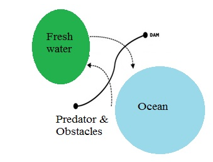Figure 1: Salmon migrating path

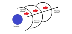Figure 2: Salmon migrating approach model

Figure 3: Computational sequences of ASTA

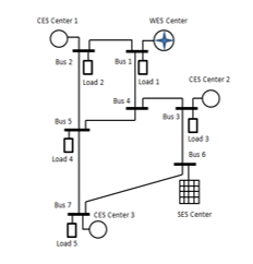Figure 4: Hybrid energy system model

Table 1: Designed Hourly Demands

Hours	MW	Hours	MW
01.00	272.50	13.00	786.95
02.00	278.81	14.00	818.13
03.00	302.29	15.00	753.83
04.00	435.45	16.00	401.49
05.00	532.67	17.00	440.37
06.00	569.59	18.00	603.54
07.00	574.16	19.00	646.96
08.00	617.78	20.00	573.33
09.00	617.93	21.00	557.76
10.00	668.49	22.00	478.80
11.00	808.82	23.00	300.52
12.00	767.71	24.00	280.54
Total		13,088.42

In particular, Figure 4 shows the energy system model for applying ASTA and for optimizing the SQOF. The developed and standard models are very helpful to meet the problem caused by completed data of the real system and difficulty data collection on the existing operation [22], [32].  In these studies, the system consists of the CES, WES, and SES centers installed at different locations. In detail, the system covers five loads which are connected to Bus 1, Bus 2, Bus 3, Bus 4, and Bus 5. Moreover, conventional energy sources are installed at Bus 1, Bus 2, and Bus 3 whereas the WES is centered at Bus 1 and the SES is integrated to Bus 6. By considering this model and conditions, the system is optimized based on demand changes for 24 hours as provided in Table 1 with the period time operation is 24 hours. These demands also cover for the day and night peak loads.

Table 2: Individual Power Productions

Time	Conventional Generating Unit (MW)
	CES C1		CES C2		CES C3
	Unit 1	Unit 2	Unit 1	Unit 2	Unit 1
	G1	G2	G3	G4	G5
01.00	65.75	22.34	21.77	24.40	26.98
02.00	58.06	28.74	25.00	27.78	26.49
03.00	64.27	37.72	37.43	22.63	29.06
04.00	89.87	89.72	84.27	38.33	37.21
05.00	127.16	85.70	71.48	85.07	73.56
06.00	133.42	75.05	79.94	75.32	75.02
07.00	133.74	72.76	76.86	77.47	87.10
08.00	149.42	79.68	85.00	63.75	93.10
09.00	137.76	73.57	89.19	71.75	77.55
10.00	220.36	70.42	72.17	67.85	72.31
11.00	257.25	98.50	97.34	98.83	98.90
12.00	254.38	84.62	94.91	82.94	86.13
13.00	259.31	91.36	91.23	84.94	92.13
14.00	268.31	94.62	98.92	95.84	97.28
15.00	239.49	82.72	96.54	88.84	83.35
16.00	100.16	49.21	46.27	42.02	23.58
17.00	103.99	59.12	80.98	35.00	24.62
18.00	187.57	74.37	74.37	78.78	65.11
19.00	187.56	81.73	84.41	87.17	83.90
20.00	187.51	78.21	77.96	67.25	72.88
21.00	166.58	73.98	75.74	73.14	73.78
22.00	125.94	68.77	61.35	61.14	64.78
23.00	62.52	31.52	32.29	33.54	31.24
24.00	53.65	35.52	25.00	28.10	27.87
Total	3634.03	1639.95	1680.42	1511.88	1523.93

 

4. Result

In this section, the IEMC is presented dynamically within 24 hours and it is optimized using ASTA. The 24 hours operation common approaches for the existing operation is based on all integrated energy producers [7], [27]. By considering ASTA’s parameters detailed in Section 3, the energy mixed producer is determined optimally as given in Table 2 for the optimal power production. Technically, this table shows the individual power commitment of the energy sources of the CES while the WES and SES are considered free for the natural energy sources as given in Table 3. From this table, it is known that this table informs the scheduled power production for 24 hours determined totally in 9,990.21 MW with the power fluctuation and contribution are illustrated in Figure 5 and Figure 6. These aspects are inlined with many previous works that the system has been delivered in variable portions associated with demand changes at the energy consumers [33].

According to Table 2 and Table 3, it is also known that all conventional generations have produced power outputs in different capacities. These different capacities show the generated participation in the system for supporting the provided energy for the load demand as reported in [14], [15]. The energy contributors cover all centers as detailed in both tables. In total, Center 1 takes a role in the highest power production of around 5,273.98 MW. Furthermore, the lowest contributor is supported by the CES Center 3 in 1,523.93 MW. By considering the IRES, Table 3 presents all penetrations within 24 hours for the SES and the WES. This penetration is very important to measure a renewable energy inclusion into the existing system with a certain portion of the participants to control the total energy production [10]. These penetrations cover hourly operations, totally, the system is penetrated in 1,450.00 MW of the SES and 2,522.93 MW of the WES. In detail, the system provides around 13,870.21 MW with the discharged pollutant of the CES is listed in Table 4 for all operating times. This emission is categorized in the produced emission, permitted emission, and over emission. As given in Table 4, the total emission is produced in 19,662.34 kg where the pollution is allowed around 8,491.65 kg based on standard emission. In addition, the system has 11,170.69 kg of the over emission during existing energy sources. It means that the system should be maintained to keep the emission level.

Table 3: Effective Balanced Power Contributions

Hour	CES (MW)	SES (MW)	WES (MW)	Total (MW)
01.00	161.24	50.00	75.00	286.24
02.00	166.07	50.00	75.00	291.07
03.00	191.11	50.00	75.00	316.11
04.00	339.40	50.00	75.00	464.40
05.00	442.97	50.00	75.00	567.97
06.00	438.75	50.00	112.50	601.25
07.00	447.93	50.00	112.50	610.43
08.00	470.95	75.00	112.50	658.45
09.00	449.82	75.00	127.50	652.32
10.00	503.11	75.00	127.50	705.61
11.00	650.82	85.00	127.50	863.32
12.00	602.98	85.00	127.50	815.48
13.00	618.97	85.00	127.50	831.47
14.00	654.97	85.00	127.50	867.47
15.00	590.94	85.00	127.50	803.44
16.00	261.24	50.00	112.50	423.74
17.00	303.71	50.00	112.50	466.21
18.00	480.20	50.00	112.50	642.70
19.00	524.77	50.00	121.05	695.82
20.00	483.81	50.00	116.76	650.57
21.00	463.22	50.00	134.36	647.58
22.00	381.98	50.00	100.48	532.46
23.00	191.11	50.00	63.91	305.02
24.00	170.14	50.00	43.87	264.01
Total	9,990.21	1,450.00	2,522.93	13,963.14

In particular, an energy balance is one of the important parameters in the system operation while the energy should be used in the final users at various types of appliances based on the power capacities [11].  In this case, the energy consumption has corresponded to individual power productions. This aspect is also used to present individual contributors to the power unit commitment. In these works, individual performances of the energy producer unit are presented in Figure 7 and Figure 8 covered hourly power production changes and hourly power fluctuations. In total, the IEMC produces 9.990.21 MW with the power produced performances as given in Figure 7 and Figure 8. Figure 7 shows the fluctuation of power productions for the CES from the present to the next hours associated with the own scheduled power production. The detailed contributor to the power plants is presented in Figure 7. This figure informs that the highest contributor comes from G1 of the CES Center 1. Moreover, the IEMC also emits the total over emission of around  19,662.34 kg whereas the IRES penetrates are given in Figure 8. This figure illustrates the hourly penetration to the system covered in 24 hours for the WES and the SES. In addition, the CES is performed in Figure 7 for the hourly power production during an existing system to supply the load center.

Table 4: Emission Discharge of the CES

Hour	Production (kg)	Permission (kg)	Over Emission (kg)
01.00	164.08	137.05	27.03
02.00	174.84	141.16	33.68
03.00	206.05	162.44	43.61
04.00	551.79	288.49	263.3
05.00	829.62	376.52	453.1
06.00	805.44	372.94	432.5
07.00	852.91	380.74	472.17
08.00	922.52	400.31	522.21
09.00	849.31	382.35	466.96
10.00	1,009.86	427.64	582.22
11.00	1,680.31	553.2	1127.11
12.00	1,450.49	512.53	937.96
13.00	1,522.32	526.12	996.2
14.00	1,709.01	556.72	1152.29
15.00	1,392.26	502.3	889.96
16.00	307.68	222.05	85.63
17.00	438.46	258.15	180.31
18.00	915.03	408.17	506.86
19.00	1,101.78	446.05	655.73
20.00	923	411.24	511.76
21.00	858.86	393.74	465.12
22.00	603.34	324.68	278.66
23.00	209.17	162.44	46.73
24.00	184.21	144.62	39.59
Total	19,662.34	8,491.65	11,170.69

Figure 5: Hourly power fluctuation

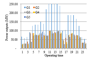Figure 6: Hourly individual power production

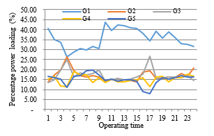Figure 7: Hourly power production of the CES

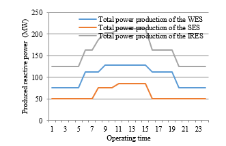Figure 8: Hourly power penetration of the IRES

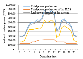Figure 9: Hourly power balance performance

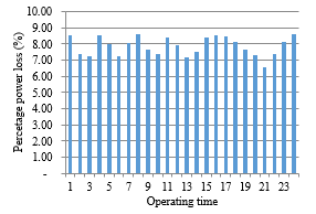Figure 10: Total reactive power loss performances

By considering the 24 hours operation, the power balance is detailed in Figure 9. This figure shows all participation of the energy producers balanced to the total hourly demand. It is also known that the main power producers are covered in conventional energy producers. In addition, the IRES is operated to support this optimal condition which is linked to the hourly composition. In these works, another problem is given in the power loss as depicted in Figure 10 designed for the 24 hours operation. The system has fluctuated power losses for the 24 hours operation associated with day and night loads.

5. Conclusion

As stated earlier, the composition of the energy mix is integrated by considering integrated renewable energy sources and various technical requirements, as well as environmental constraints. The formula is outlined in a computational problem that is searched using the Artificial Salmon Tracking Algorithm to get the optimal composition for 24 hours. The calculation results show that dynamically the part of the energy produced is affected by IRES as given in solar and wind energy sources for 24-hour operations. In addition, ongoing conventional energy producers contribute with different capacities to support individual commitments to the production of power units. Furthermore, from these works, the implementation of real algorithms for large systems is suggested for future work in line with the placement of distributed renewable energy.

Acknowledgment

The authors gratefully acknowledge the support of the DRPM Research Grant 2019, Ministry of Research, Technology and Higher Education, Indonesia.

1.  M. Malekidelarestaqi, A. Mansouri, and S. F. Chini, “Electrokinetic energy conversion in a finite length superhydrophobic microchannel,” Chem. Phys. Lett., vol. 703, pp. 72–79, Jul. 2018.
2.  Z. Dimitrova and F. Maréchal, “Energy integration on multi-periods and multi-usages for hybrid electric and thermal powertrains,” Energy, vol. 83, pp. 539–550, Apr. 2015.
3. X. Zhang, Z. Wang, H. Shen, and Q. J. Wang, “Dynamic contact in multiferroic energy conversion,” Int. J. Solids Struct., vol. 143, pp. 84–102, Jun. 2018.
4.  P. Cuffe and A. Keane, “Visualizing the Electrical Structure of Power Systems,” IEEE Syst. J., vol. 11, no. 3, pp. 1810–1821, Sep. 2017.
5. M. Bhoye, M. H. Pandya, S. Valvi, I. N. Trivedi, P. Jangir, and S. A. Parmar, “An emission constraint Economic Load Dispatch problem solution with Microgrid using JAYA algorithm,” in 2016 International Conference on Energy Efficient Technologies for Sustainability (ICEETS), 2016, pp. 497–502.
6. A. Rabiee, B. Mohammadi-Ivatloo, and M. Moradi-Dalvand, “Fast Dynamic Economic Power Dispatch Problems Solution Via Optimality Condition Decomposition,” IEEE Trans. Power Syst., vol. 29, no. 2, pp. 982–983, Mar. 2014.
7.  Y. Shang, S. Lu, J. Gong, R. Liu, X. Li, and Q. Fan, “Improved genetic algorithm for economic load dispatch in hydropower plants and comprehensive performance comparison with dynamic programming method,” J. Hydrol., vol. 554, no. Supplement C, pp. 306–316, Nov. 2017.
8. M. El-Shimy, M. A. Attia, N. Mostafa, and A. N. Afandi, “Performance of grid-connected wind power plants as affected by load models: A comparative study,” in 2017 5th International Conference on Electrical, Electronics and Information Engineering (ICEEIE), 2017, pp. 1–8.
9. L. Wang, W. Liu, D. Malcolm, and Y. F. Liu, “An Integrated Power Module Based on Power-system-in-inductor Structure,” IEEE Trans. Power Electron., vol. PP, no. 99, pp. 1–1, 2017.
10.  Y. Li, S. Miao, X. Luo, and J. Wang, “Optimization model for the power system scheduling with wind generation and compressed air energy storage combination,” in 2016 22nd International Conference on Automation and Computing (ICAC), 2016, pp. 300–305.
11.  L. Labib, M. Billah, G. M. S. M. Rana, M. N. Sadat, M. G. Kibria, and M. R. Islam, “Design and implementation of low-cost universal smart energy meter with demand side load management,” Transm. Distrib. IET Gener., vol. 11, no. 16, pp. 3938–3945, 2017.
12.  T. J. Hammons, “Europe: transmission system developments, interconnections, electricity exchanges, deregulation, and implementing technology in power generation with respect to the Kyoto protocol,” in 39th International Universities Power Engineering Conference, 2004. UPEC 2004., 2004, vol. 3, pp. 1251–1257 vol. 2.
13. S. Walker, K. W. Hipel, and T. Inohara, “Strategic analysis of the Kyoto Protocol,” in 2007 IEEE International Conference on Systems, Man and Cybernetics, 2007, pp. 1806–1811.
14.  N. Ghorbani, E. Babaei, and F. Sadikoglu, “Exchange market algorithm for multi-objective economic emission dispatch and reliability,” Procedia Comput. Sci., vol. 120, pp. 633–640, 2017.
15.  Y. Di, M. Fei, L. Wang, and W. Wu, “Multi-objective Optimization for Economic Emission Dispatch Using an Improved Multi-objective Binary Differential Evolution Algorithm,” Energy Procedia, vol. 61, no. Supplement C, pp. 2016–2021, Jan. 2014.
16. L. T. Al Bahrani and J. C. Patra, “Orthogonal PSO algorithm for economic dispatch of thermal generating units under various power constraints in smart power grid,” Appl. Soft Comput., vol. 58, no. Supplement C, pp. 401–426, Sep. 2017.
17. P. Boonserm and S. Sitjongsataporn, “A robust and efficient algorithm for numerical optimization problem: DEPSO-Scout: A new hybrid algorithm based on DEPSO and ABC,” in 2017 International Electrical Engineering Congress (iEECON), 2017, pp. 1–4.
18.  A. Shenfield, D. Day, and A. Ayesh, “Intelligent intrusion detection systems using artificial neural networks,” ICT Express, May 2018.
19.  B. Chowdhury and G. Garai, “A review on multiple sequence alignment from the perspective of genetic algorithm,” Genomics, vol. 109, no. 5, pp. 419–431, Oct. 2017.
20. C. L. Bottasso, S. Cacciola, and J. Schreiber, “Local wind speed estimation, with application to wake impingement detection,” Renew. Energy, vol. 116, pp. 155–168, Feb. 2018.
21. G. Cervone, L. Clemente-Harding, S. Alessandrini, and L. Delle Monache, “Short-term photovoltaic power forecasting using Artificial Neural Networks and an Analog Ensemble,” Renew. Energy, vol. 108, pp. 274–286, Aug. 2017.
22.  K. B. Debnath and M. Mourshed, “Forecasting methods in energy planning models,” Renew. Sustain. Energy Rev., vol. 88, pp. 297–325, May 2018.
23. N. Tutkun, O. Can, and A. N. Afandi, “Low cost operation of an off-grid wind-PV system electrifying residential homes through combinatorial optimization by the RCGA,” in 2017 5th International Conference on Electrical, Electronics and Information Engineering (ICEEIE), 2017, pp. 38–42.
24.  A. N. Afandi, I. Fadlika, and Y. Sulistyorini, “Solution of dynamic economic dispatch considered dynamic penalty factor,” in 2016 3rd Conference on Power Engineering and Renewable Energy (ICPERE), 2016, pp. 241–246.
25.  F. P. Mahdi, P. Vasant, V. Kallimani, J. Watada, P. Y. S. Fai, and M. Abdullah-Al-Wadud, “A holistic review on optimization strategies for combined economic emission dispatch problem,” Renew. Sustain. Energy Rev., vol. 81, no. Part 2, pp. 3006–3020, Jan. 2018.
26. A. N. Afandi, “Weighting Factor Scenarios for Assessing the Financial Balance of Pollutant Productions and Fuel Consumptions on the Power System Operation,” Wseas Trans. Bus. Econ., vol. 14, 2017.
27.  A. N. Afandi, Y. Sulistyorini, G. Fujita, N. P. Khai, and N. Tutkun, “Renewable energy inclusion on economic power optimization using thunderstorm algorithm,” in 2017 4th International Conference on Electrical Engineering, Computer Science and Informatics (EECSI), 2017, pp. 1–6.
28.  A. N. Afandi et al., “Designed Operating Approach of Economic Dispatch for Java Bali Power Grid Areas Considered Wind Energy and Pollutant Emission Optimized Using Thunderstorm Algorithm Based on Forward Cloud Charge Mechanism,” Int. Rev. Electr. Eng. IREE, vol. 13, no. 1, pp. 59–68, Feb. 2018.
29.  C. C. Columbus and S. P. Simon, “A parallel ABC for security constrained economic dispatch using shared memory model,” in Controls and Computation 2012 International Conference on Power, Signals, 2012, pp. 1–6.
30.  Denglijun, Zipeng, Anning, Shaoguanghui, Xuxingwei, and Houkaiyuan, “Empirical analysis on model and parameters of grid-connected Direct-driven Wind Turbine Generators in transient stability computation,” in 2014 China International Conference on Electricity Distribution (CICED), 2014, pp. 1184–1189.
31. S. Chatterjee and S. Mandal, “A novel comparison of gauss-seidel and newton- raphson methods for load flow analysis,” in 2017 International Conference on Power and Embedded Drive Control (ICPEDC), 2017, pp. 1–7.
32.  L. Jodar, J. R. Torregrosa, J. C. Cortés, and R. Criado, “Mathematical modeling and computational methods,” J. Comput. Appl. Math., vol. 330, pp. 661–665, Mar. 2018.
33.  M. EL-Shimy, N. Mostafa, A. N. Afandi, A. M. Sharaf, and M. A. Attia, “Impact of load models on the static and dynamic performances of grid-connected wind power plants: A comparative analysis,” Math. Comput. Simul., Feb. 2018.

(Click Here)

(Click Here)