1. Introduction

In an enterprise Wlan network, the controller is the central component of the network architecture. The controller manages all the Wifi access points (APs) and provides their radio configuration: channel and transmit power. The controller plays another important role in Wlan integration to other parts of the enterprise network: Local Area Network (LAN), Wide Area Network (WAN), internet, and Datacenter Network (DCN), where application servers reside.

Processing the radio plan is the task of RRM functional architecture block of the controller. It helps minimize cochannel interference and efficient use by APs of the spectrum, thus, optimizing the latter transmit opportunity. Then, how does RRM decide on what channel an access point should use, and at what transmit power?

To build an efficient radio plan that maximizes the network capacity, the controller needs data from APs, Wifi clients or devices (WDs), wired network devices, and servers. This data is what pertains to the quality of the radio interface and client overall experience when accessing the services. However, this information is not sufficient to hint on the whole coverage quality such as the interference at any point in the coverage area. It is only limited to some coverage points, APs and WDs, that are able to monitor the radio interface and report real radio measurements.

To overcome this limitation, either we place sensors everywhere, which is not feasible in an enterprise network (economically and technologically), or model the coverage area. The modelization effort could be done in a laboratory context, by vendors for example, to provide strict recommendations that customers may follow to build their networks. This approach works in common situations. But it requires a lot of engineering effort and monitoring to maintain the network at an optimal condition. In some situations, it may just not work or false the transmit opportunity estimation. For the rest of this work, this approach is referred to as static RRM (sRRM). The third alternative is to allow the controller to do more complex real-time processing without any or very few preconfigured settings and find out the suitable RRM configuration to apply. This approach is the focus of this study and will be referenced as dynamic RRM, or dRRM.

A controller, that supports dRRM, does not rely on preconfigured settings in hardware or software to decide on how to modify the radio plan to meet the utility function. In dRRM, even the system parameters are processed to optimize the network capacity, which is different from sRRM. However, the advantage of dRRM comes at a high price in terms of time, system resources consumption to process the whole network coverage and, adaptation to frequent changes. In this work, we present our dRRM optimization solution that builds on concepts from the Machine Learning (ML) field. Our solution is built on a novel and realistic per-Beam coverage representation approach that is different from related-work encountered research approaches that we discuss later.

In Section 2, we present how related work, research and vendors, process RRM. In Section 3, we present our dRRM solution (that is not sRRM) and compare it to the vendor solution in processing the radio coverage. Before we state the problem in Section 5, and the presentation of our solution in Section 6, we introduce in Section 4, some important facts about Wlan network design, coverage representation models and important machine learning concepts. Section 7 is dedicated to the evaluation of our optimization, before we conclude.

This paper is an extension of the work originally presented in the 2018 15^th International Conference on Electrical Engineering, Computer Science and Informatics [1].

2. RRM Related Work

In this section, we discuss RRM approaches from research and vendors of the Wifi market such as Cisco, Aruba-HPE, etc. as they pertain to enterprise Wlan networks. We are interested in algorithms that operate the APs transmit power to maximize the network capacity or optimize radio resource usage. An algorithm is different from another when the used variables are different.

For simplification, we discuss a mono channel condition. This work could then, be easily extended to a multi-channel condition.

2.1     In Research

The first category of approaches concentrate on lower-layer constraints: co-channel interference, physical interface and MAC performance.

The authors in these works [2, 3, 4], modeled the coverage area per-range: transmit, interference, and not-talk ranges, using a circular or disk pattern. The way this model represents the coverage is common but may not hint on some opportunities to transmit as discussed in this work [5].

The author in this work [6], focused instead on the interaction that an AP may have with its neighboring AP. The result is a per-zone, Voronoi zone, negotiated coverage pattern. This model is difficult to put into practice technologically and economically as it was discussed in [5] and [7]. Both models: per-zone and per-range, do not consider upper layer constraints.

Another set of similar works tackle the issue from a power saving perspective. The authors in [8] build their on-demand Wlan approach on the observation of idle APs that have no clients associated. The Wlan controller manages the activation or not of an AP.

The second category of approaches tackles the issue from an upper-layer perspective for applications such as FTP, HTTP. This work [9], as an example, presented an interesting idea to find out a suitable power, or RRM, scheme, that may optimize the application performance. It is a per-experience approach that requires a huge amount of data, to be put into practice. In addition, it is very dependent on the coexistent individual application’s behavior. Another challenge is to be able to determine when the physical layer is responsible for the observed performance rather than the application one. Works like [10] use concepts from the Game theory, a powerful tool, to model the interactions between APs. These concepts are applied to the user perception of the QoS it receives. The same limitation of the previously cited work applies to this one also.

The third category tackles the problem from an interprotocol cooperation point of view like in this example [11]. Making the protocols aware of each other is a good strategy to find an optimum inter-protocol negotiated power scheme that optimizes the performance of each of them individually. It is an idealistic scheme, difficult to put into practice technologically and economically, concerning vendors offering. Let us imagine the integration of a Wifi and a Bluetooth network. The impact of a Wifi AP on a Bluetooth piconet is very important but not the opposite. Then, as an example, it is necessary to find out a way to provide the network controller (for both Wifi and Bluetooth) with the necessary feedbacks so it can adjust the Wifi network power plan to allow a Bluetooth network optimum operation. This would require important data transfers (and power consumption) from the Bluetooth network to the controller, which is very difficult to implement, by design of the Bluetooth devices..

2.2     Vendor Solutions

The approach or theoretical background, behind the vendors’ implementations, is hidden in general for commercial purposes; they only provide the settings (recommendations).

Cisco Transmit Power Control (TPC) algorithm, that is a part of Cisco RRM, processes, at each AP, the desired transmit power hysteresis, T x_{Hysteresis,Current}, that is equal to the sum of the current transmit power (initially at maximum), T x_Current, and the difference between the power threshold, T x_{T hresh}, and RSSI^3rd, the third neighbor reported RSSI. If the difference between the processed power and the current one, T x_HysteresisT hresh, is at least 6dBm, then the current power must be reduced by 3db (by half). We should then wait for 10 minutes before re-attempting another calculation. Details about this implementation are given in [12].

Aruba-HPE adopts another strategy. The Adaptive Radio Management (ARM) algorithm maintains two measures for every channel: a coverage index, cov_idx, and an interference index, if er_idx. The decision of increasing or decreasing the transmit power level on a given channel is based on the processed coverage index as compared to the “ideal” coverage index, noted cov_idx,ideal, and “acceptable” coverage index, cov_{idx,acceptable}, for instance. As a general rule, the current coverage index should be greater than cov_{idx,acceptable} and equivalent to cov_idx,ideal. Coverage index, cov_idx, corresponds to the sum of two variables : x and y. x is the weighted average of all other APs SNR as being measured by the current AP. y is the weighted average of the processed x variables by other APs from the same vendor and on the same channel. The same thing applies to if er_idx processing. Details of this calculation are in [13].

Fortinet Auto Power that is a part of ARRP, Automatic Radio Resource Provisioning, solution, works by reducing automatically the transmit power if the transmit channel is not clear. From the corresponding documentation [14], it is an alternative to manually limiting the number of neighbors per channel (less than 20) by adjusting the transmit power level.

3. Our Dynamic RRM Solution

Our WLCx dynamic RRM solution is based on the per-Beam coverage representation we discuss in the upcoming section. Our solution is ”dynamic” because even the parameters’ values change: the optimum number of the supported directions per AP, in the case of the WLC2 variant of our solution, as an example. The workflow in Figure 1, describes how our solution works.

Our solution runs three algorithms: TDD (Discovery), TDM (Map) and TDO (Opportunity). After initialization, TDD optimizes the number of supported directions per AP by reducing the power level and doubling the initial number of directions until all neighbors are discovered and at almost one neighbor is discovered per AP direction. Based on information from TDD, TDM categorizes the coverage area points into categories that hints on how these points appear on APs directions. Each category is assigned a cost to hint on its probability to get a fair transmit opportunity. The TDO processes each coverage point opportunity to transmit, taking into account data from TDM and SLA (upper-layer input).

We simulate, using Matlab 2019a, two variants of our WLCx solution: WLC1 and WLC2. In WLC1, all APs share the same optimal number of supported directions and transmit at the same power level. In WLC2, the APs process the same optimal number of the supported directions but may use different transmit power levels per AP. In the same simulation, we compare both WLCx variants to vendor implementation: Cisco. We evaluate models based on their performance at processing the coverage and time this processing takes.

The coverage processing performance, P r(), of a given model, m, is calculated in (1). I(), H() and O() are the model processed interference, number of coverage holes and transmit opportunity, respectively.

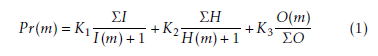The performance calculation in (1), is the weighted sum of relative interference, opportunity and coverage holes in each model. The weights K₁, K₂ and K₃, hints on how important is the processing of interference, opportunity or holes, to the performance of a given model. For the rest of our study, we consider that all variables are of equal importance then, K₁ = K₂ = K₃ = 1.

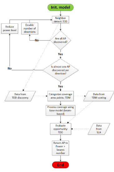Figure 1: Our WLC dRRM solution workflow

The diagram in Figure 2, shows the performance of models after 10 iterations of the same simulation. Each simulation corresponds to a random distribution of a set of 30 APs and 100 WDs. We check that our WLC2 solution variant performs better than Cisco and WLC1. The Cisco model performance is comparable to WLC1. The processing time of models is represented in Figure 3. The models have a comparable processing time for a large number of the same simulation iterations.

In work [5], we discuss our WLC2 dRRM solution. For further details about our solution, refer to [7] work that is an extension of the previous one.

4. Theoretical Background

Before we dive into the description of the problem, let us recall some facts about Wlan enterprise network architecture design, the importance of coverage representation for radio planning, and NURBS surfaces concepts that are the foundation of our NURBS optimized WLCx dRRM solution.

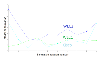Figure 2: Performance of models after 10 simulations of the network of 30 APs and 100 WDs.

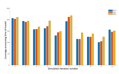Figure 3: Processing time of models after 10 simulations of the network of 30 APs and 100 WDs.

4.1      Wifi Unified Architecture

In a standalone AP-based Wifi architecture, the network capacity does not scale with dense and frequently changing radio environments. To optimize the network capacity, some kind of coordination and control, distributed or centralized, is needed. In UWA, Unified Wifi Architecture, a WLC, Wireless LAN Controller, acts as a repository of APs intelligence, runs routines to plan radio usage, provides an interface to wired network, etc. and guarantees conformance to policies: QoS and Security, domain-wide, including LAN, MAN, WAN, and DCN, network parts. A typical enterprise Wlan architecture is given in Figure 4. Two market-leading implementations of such WLCs are the Cisco 8540 Wireless Controller and the Aruba 7280 Mobility Controller. The rest of our study focuses on Cisco implementation.

In Figure 4, the APs are located nearest to Wifi clients, WDs. All APs are connected to the LAN and are associated, via Virtual Private Networks (VPN), or tunnels, to the controller, WLC, located at the Datacenter, in a Hub and Spoke architecture. Depending on the network size and requirements, the controller may be located at the same location as the APs. To build an association, an AP should be able to join the controller, via MAN, WAN or internet. After the AP’s successful association to the controller, the WDs start their association process that includes authentication, to the corresponding Wlan. Then the WDs access the network resources behind the controller or in some configurations, behind the APs (in FlexConnect or Local Switched mode).

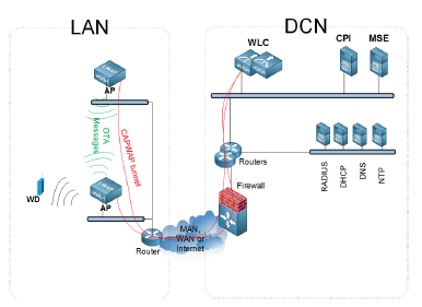Figure 4: A Wifi unified architecture example topology

WLC receives information about the network from three sources: the wired path toward the datacenter, the radio interface counters of each associated AP, and OTA, Over-The-Air,

AP-to-AP wireless messages over a dedicated low speed radio. In the case of Cisco, two protocols are available for exchanging data between APs, and between APs and WLC:

• Control and Provisioning of Wireless Access Points (CAPWAP) protocol is used by the APs to build associations to the RF group leader WLC and for control information and data exchange.
• Neighbor Discovery Protocol (NDP) allows the APs to exchange Over-The-Air (OTA) messages that carry standard, per-vendor proprietary control, and management information.

In addition to these protocols, Cisco APs have on-chip features such as CLIENTLINK and CLEANAIR. CLEANAIR enables the APs to measure real-time radio characteristics and send them to the controller via the already established CAPWAP tunnels. Cisco appliances such as Cisco Prime Infrastructure (CPI) and Mobility Services Engine (MSE), shown in Figure 4, extend the capability of this feature to process analytics on Wifi client presence, interfering devices management and heatmaps processing. CLIENTLINK version 4.0, is the Cisco at AP-level implementation of MU-MIMO IEEE 802.11ac beamforming. It works independently of CLEANAIR after the assessment of the quality of the channel. In this scheme, an AP sends a special sounding signal to all its associated WDs, which report, back to this AP, their signal measurement. Based on these feedbacks, the AP, and not the controller, decides on how much steering toward a specific WD is needed to optimize the energy radiation.

4.2     Radio Coverage Representation Models

We categorize the related-work coverage representation models into three categories: Range-based, Zone-based and Beambased. In the upcoming subsections, we describe each of them and discuss their limitations.

In the Range-based category of models, it is common to represent an AP’s wireless coverage such as: a transmission, interference or no-talk range. These ranges processing is based on the estimation of the distance between the AP and a receiving point P (AP or WD). Further, this category of coverage representation models, consider that an AP’s coverage pattern is omnidirectional, with the geometric shape of a circle or a disk, centered at the AP, like in Figure 5. In this scheme, the interference, for example, at any given point is approximated by the weighted intersection of all interfering devices patterns at this point.

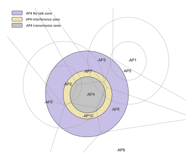Figure 5: A range-based coverage representation example

In the Zone-based category of models, an AP coverage is a function of its transmission characteristics: channel, power level, etc., but depends also on the neighboring APs. The result of this is that the transmission shape is no more a solid circle but a convex polygon with straight sides. Each straight side defines a borderline that separates two neighboring APs’ transmission ranges. The more an AP transmit power is strong, the more the borderline with its neighboring APs is far. Further, it is important to note that a point in a transmission zone of one AP could not be in another AP’s transmission zone. An example of Zone-based AP’s wireless coverage is represented in Figure 6. In this scheme, the interference caused by the transmission ranges in the previous model, is completely canceled. Only the interference caused by the other ranges: interference, and no-talk ranges, is present.

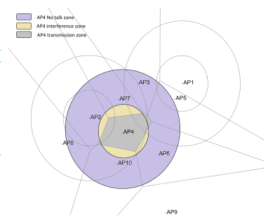Figure 6: A zone-based coverage representation example

The previous two models: Range and Zone-based, come with these limitations:

• both models are limited to consider that the strength of interference is only inversely proportional to the distance (or quadratic) of an AP from interfering neighbors,
• both models would interpret an increase in a transmis-sion power level as an expanded reach in all directions: uniformly in case of Range-based models but depending on neighboring APs in the case of Zone-based ones,
• a point could not be in two transmission ranges of two different APs at the same time in Zone-based models,
• both models would interpret falsely obstacles to the signal propagation, as a weaker signal from an AP in the context of indoor Wlans does not mean necessarily that this AP is out of reach,
• alternatively, a stronger signal from an AP does not mean necessarily that this AP is at reach: it may be guided or boosted under some conditions.

The consequences of these limitations, the adoption of a Range or Zone-based like representation model of coverage, and regardless of the RRM solution that is built upon, is to false our transmit opportunity processing and misinterpret some phenomena encountered in the specific context of indoor enterprise Wlans.

To overcome the limitations of the previous models, our Beam-based coverage representation, defines for each AP a number of directions over which it may transmit. Depending on the number of directions, their order and transmit power levels, an AP may be able to mimic a Range or Zone-based scheme. The Figure 7, shows a per-Beam coverage pattern example. In this pattern, the APs have an equal number of directions, equal to eight, that are uniformly distributed and of equivalent transmit power. In works [5, 7], we discussed in detail how per-Zone and per-Range representation models are generalized to per-Beam representation and how our representation model could solve previous models limitations such as : per direction transmit power control, hole coverage reduction, obstacle detection, client localization and transmit opportunities maximization.

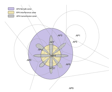Figure 7: A beam-based coverage representation example

4.3      Machine Learning Regression Models

In his book [15], Tom Mitchell describes a machine, computer program, etc. process of learning when from an experience ”E” with respect to some task ”T” and some performance measure ”P” of this task, its performance on ”T”, as measured by ”P”, improves with experience ”E”.

A simple form of this learning, focus of this work, is described as ”supervised” learning. In this learning, the right answers to some input or training data, are provided in advance. Based on this training data, the inputs and corresponding outputs or ”truth”, the learning algorithm model parameters are processed such as to minimize the error between the predicted outputs and the observed ”truth” on the training set.

This ”trained” learning, also called hypothesis, is indeed a function that is built using the previously optimized model parameters. This function maps the input variables or features to a predicted outcome.

Supervised learning algorithms could be further classified by the nature of the outcome they work on. If the outcome is continuous, then ”regression” models are more suitable. For categorical or discrete outcome values, ”classification” algorithms are more suitable.

In our study, we work on outcomes that are continuous, and then we focus solely on regression models. Many types of regression models exist including: linear regression models (LR), regression trees (RT), Gaussien process regression models (GPR), support vector machines (SVM), and ensembles of regression decision trees (BDT).

To choose between models, we compare their Root Mean Square Error (RMSE) validation score. In all the simulations of our work, we observe that Coarse Gaussian SVM and BDT score the best RMSE scores. For the rest of our study, we focus solely on these two models.

Furthermore, SVM and BDT methods represent two distinct algorithm general approaches. In the following subsections, we introduce the important differences in these two approaches.

4.3.1      Support Vector Machines

In SVM, the samples are separated into categories. The idea of this algorithm is to find the maximum gap between these categories. The samples that help find this separation are called support vectors. Each support vector is seen as a dimensional data and the goal of the algorithm is to find the best hyperplane in terms of margin that separates these vectors.

In this work, we use SVM to resolve a linear regression problem. We use a variable that controls the trade-off between the classification errors and the size of the margin.

This method corresponds to a soft-margin SVM.

4.3.2      Bagged Decision Trees

Bagging decision trees (BDT) is a meta-algorithm that builds on an ensemble of algorithms that run independently from each other. Each algorithm, called bootstrap, obtains a different result. The result of the meta-algorithm corresponds to the average of the bootstraps individual results. In our case, a bootstrap algorithm may correspond to a simple regression.

The initial training set has n elements. BDT generates, from this set, m new subsets of size n⁰ less than the original set size. If n is equal to n⁰ and n is very big, the probability that each subset has unique values from the initial set is almost 63.2%, the other values are duplicated.

An example of such meta-algorithm is Classification And Regression Trees (CART). The tree operates using a metric and by classifying at each stage, the initial set, the set we are predicting the outcome for. This metric is based on Gini impurity that is calculated from the probability of a certain classification. The classes, which are used in this classification, have been identified during the training phase. In the case of a regression, the algorithm introduces the notion of the variance reduction to build the classes and the corresponding metrics.

5. Problem Description

Coverage processing includes the calculation of interference, opportunity and coverage holes, as per our Beam-based representation model, that is a generalization of the previous work models such as Range or Zone-based representation models. For the problem description, let us define:

P_i              — a coverage point.

L_j,k             — AP_j, number k direction.

C_i                 — the sensitiviy of point P_i at reception.

C_i,1 — AP to which P_i is associated, range of transmission.

C_j,2 — AP_j, interference range.

C_j,3 — AP_j, no-talk range.

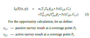
We show in (2), the interference I_B() that is calculated by WLC2, our WLCx dRRM solution variant, using Beambased representation model. The processed interference by this model at a point P_i, corresponds to the sum of the intersections, Sc(), of all APs beam patterns with C_i and their interference and no-talk ranges with C_i,1 that is the transmission range of AP_i to which the point P_i is associated.

For the opportunity calculation, let us define: s_1,i  — passive survey result at a coverage point P_i.s_2,i   active survey result at a coverage point P_i. In (3), we give the opportunity calculated by WLC2 model, using our Beam-based representation model, O_B(). The opportunity is inversely proportional to the interference calculation and hints also, on the result of surveys on the active and passive network paths: s_1,i and s_2,i. Passive surveys allow the controller to have statistics and metrics from the network devices and attached interfaces that are on the network path between the client and the server such as the number of transmit errors, number of lost packets, etc. and is generally available via protocols such: SNMP or Simple Network Management Protocol. Active surveys instead, construct traffic patterns and simulate actively the traffic between the client and the server, using protocols such as UDP or TCP, and report measurements such as delay, jitter, etc. to the controller.

The last element to include in the coverage processing, is the number of the detected coverage holes, that is given in (4). Coverage holes are evaluated at every coverage point P_i and correspond to points where the signal is insufficient to perform an accurate communication with their APs of association or the access network, if they are not already associated. holeT hesh_i is another variable that is tight to the point P_i sensitivity at reception.

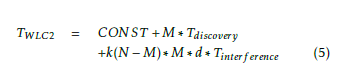
The processing of the coverage, that is done in (2), (3) and (4), is a part of the general processing of our dRRM solution variants: WLC1 and WLC2 that is described in Figure 1 workflow. We give in (5) the necessary time to process the coverage and the changes to this coverage. In (5), we neglected, for simplification, the necessary time to process the optimal number of directions that are supported by the APs and the corresponding transmit power levels. M is the number of APs and any monitoring device. T_discovery is the necessary time to run TDD and build a neighborship map. N is the number of coverage points, where the coverage must be calculated. d is the optimum processed number of directions that are supported by APs. T_{interf erence} corresponds to the necessary time to process coverage. We consider that Tinterf erence, Topportunity and T_holes, times are equivalent.

In Figure 8, we plot the processing time results of models with and without control: simplistic (Range-based), idealistic (Zone-based), WLC1, WLC2 (dRRM) and Cisco (sRRM). We notice that in general, the without-control models perform better than the with-control models due to the addition of the control part of processing. The processing times of the with-control models are equivalent but huge in comparison with the without-control models.

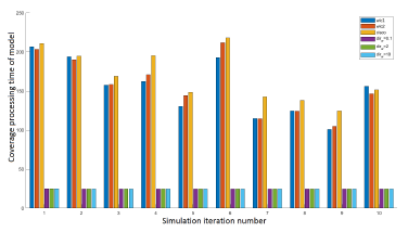Figure 8: WLC2 time in comparison with idealistic and simplistic models.

The sRRM and dRRM solutions have advantages over each other and over the without-control models, approaches but they require important processing time and resources, which is not suitable in the context of indoor dense enterprise Wlans. In the next section, we propose an optimization solution to with-control RRM models, which is based on concepts from the Machine Learning (ML) field: SVM and BDT. To stick with the aim of this work, we apply this optimization to the example of our dRRM WLC2 solution, but it is easily applicable to the other approaches.

6. MLR-based Optimization Solution:

Our solution is written and simulated in Matlab program M-WLC2   ming language. Further work would consider the implemen-tation of our solution on Linux-based APs and test its performance in a real laboratory setup. In Figure 10, the detailed

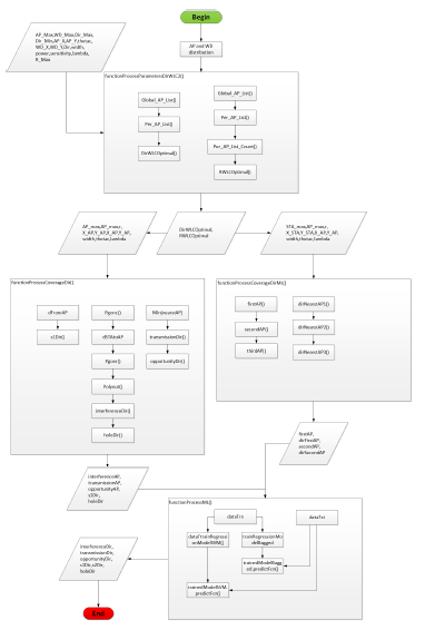Figure 10: Our ML-WLC2 solution software architecture

In this section, we present the details of our solution. We dedescription of the software architecture of our solution. The scribe the general workflow of our solution, how the training functionProcessML() module is responsible of processing the set is chosen and the criteria that allows us to choose between different data sets, training of the models and of the predicmodels: RMSE validation score. At the end of this section, we tion of the outcomes.

present the new processing time of our solution.

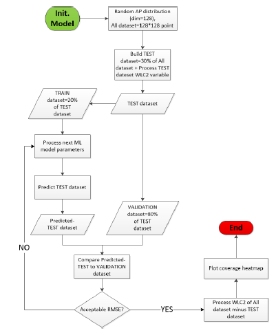Figure 9: Our ML-WLC2 solution workflow

list of neighboring AP, the second AP of association, the corresponding direction of transmission, and so on. The list may be augmented by any relevant information or feature that may have an impact on the phenomenon under study (the interference, in our case).

6.3      RMSE Validation

RMSE stands for Root Mean Square Error. It measures the error between the predicted outcome using the trained model and the truth. The truth in our case is the real measures that were reported by the network APs, WDs, and sniffers.

An important number of tests, the same simulation of the previous networks, allowed us to choose SVM and BDT models. These models score an average of 16.03 and 14.75 points respectively.

Based on the historical results, we set the acceptable RMSE validation score for a model to be accepted in processing the remaining overall dataset points, as it was described in the workflow of Figure 9.

In addition to the RMSE validation score, we use statistical results and visual observations of the heatmap to validate the precision of the outcome.

6.4     Time

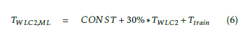
The total required processing time of our M-WLC2 solution is given in (6). The total time is the sum of the required time to train the model, T_train, and the time to process the validation set, 30% ∗ T_WLC2, where T_WLC2 is the total time required to process WLC2 solution model coverage. In case the training set points report the measurement in real-time, this time is very negligible.

7. Evaluation

In this section, we evaluate the predictions accuracy and the required processing time of the models with and without optimization: WLC2, SVM and BDT M-WLC2.

7.1     Simulation

We simulate a network of 30 APs that are distributed randomly in a 2D plan using the Matlab built-in randperm() function.

The coverage map has a dimension of 128 points in each direction. We process a total of 128 ∗ 128 = 16,384 coverage points. Each coverage point (in red) corresponds to a potential WD. The WDs are distributed uniformly on the plan.

In Figure 11, we show the distribution of the APs and WDs in the coverage area that corresponds to this simulation. AP1 and AP2 coverage is represented using their Beam-based coverage pattern. AP14 and AP15 coverage is represented by their Range-based coverage pattern.

7.2     Processing of Area Coverage Heatmap

Before we process the coverage of the optimized models, we process the coverage of the WLC2 without optimization. In Figure 12, we show the resultant heatmap of WLC2 processing that indicates the level of interference in the coverage area.

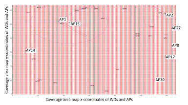Figure 11: The distribution of APs and WDs in a simulated network

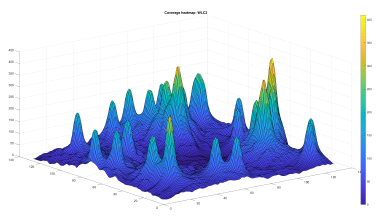Figure 12: WLC2 area coverage resultant heatmap

In Figure 13 and Figure 14, we show the result of the BDT and SVM optimized WLC2 model coverage processing, respectively. Visually we observe a strong resemblance of the three patterns.

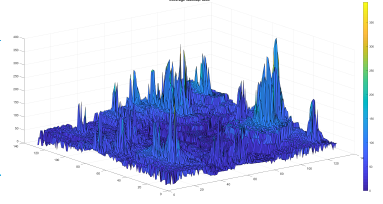Figure 13: BDT ML-WLC2 area coverage resultant heatmap

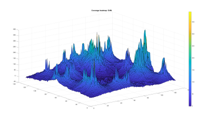Figure 14: SVM ML-WLC2 area coverage resultant heatmap

In addition to the visual resemblance, the accuracy of the models’ prediction is evaluated statistically and using the RMSE validation score. The statistical results hint on the mean, median, standard deviation in between the prediction and the WLC2 model calculated values. The performance of the models depends also on the required processing time.

7.3      Multiple Iterations of The Same Simulation

In this section, we present the results of multiple iterations of the same simulation (random distribution of APs at each iteration). In Figure 15, we draw the mean, median and standard deviation results for BDT and SVM models for 10 iterations of the same simulation.

In Figure 15, we observe that BDT presents a better mean around zero and a median slightly around five points in average. SVM shows a better median but a mean around three points in average. BDT standard deviation is twice greater in average than the SVM’s, almost 40 points in the first simulations and 30 points in the last ones.

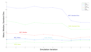Figure 15: Statistical results of 10 iterations of BDT and SVM M-WLC2 simulation

For the same simulations, we show in Figure 16, the variation of the RMSE score. We observe that the BDT solution scores the best RMSE value, almost 45 points, against the SVM model, almost 25 points, in the first simulations. In the three last simulations, the RMSE score drops to almost 25 points for BDT model and only 15 points for the SVM model.

In Figure 17, we show the required processing time of models with and without optimization. In general, we observe that the optimized models: BDT and SVM times are comparable and very negligible in comparison with WLC2 time, almost 2.5 smaller.

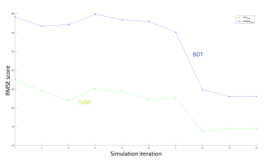Figure 16: RMSE resultats of 10 iterations of BDT and SVM M-WLC2 simulation

7.4       The Effect of Modifying The Training Set Size

In this subsection, we propose to check the effect of modifying the training set size on the optimized models performance.

In Table 1, we show the results of modifying the size of the training set in this range: 10%, 20%, 30%, 50% and 90% of the total available data set. We notice no remarkable change in statistical results in terms of mean and median in between the models when the training set is 10%, 20% and 30%. For bigger training sets, these values are getting remarkably smaller. The SVM model standard deviation decreases with the increasing training set sizes. Concerning the BDT model, we observe the opposite; the standard deviation is at its highest value when the size of the training set is 90% of the total available data set.

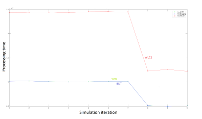Figure 17: Required processing time of 10 iterations of BDT and SVM MWLC2 simulation, training set 30% of total data set

Table 1: Effect of modifying the training set size on model performance

Var.	trnset = 10%	20%	30%	50%	90%
msvm	-3,92	-3,23	-3,25	-2,39	-2,50
mbdt	-0,27	0,18	0,11	-0,03	-0,05
medsvm	0,29	0,25	0,20	0,15	0,12
medbdt	4,69	5,66	5,37	4,87	5,45
stdsvm	23,76	20,55	19,69	16,50	16,40
stdbdt	34,93	34,75	36,90	35,90	38,91
rmsesvm	25,10	21,88	21,13	17,82	17,21
rmsebdt	34,69	34,74	37,02	36,02	38,85
tsvm	2594 ,88	3776 ,93	5291 ,24	7602 ,12	1485 1,02
tbdt	2594 ,19	3774 ,37	5286 ,25	7585 ,18	1479 3,40
twlc2	1209 1,41	1202 4,33	1280 9,81	1229 2,02	1469 0,10

In general, BDT scores better RMSE values than SVM. SVM’s RMSE score is better when the size of the training set is the smallest, 10% of the total available data set. Differently from SVM, the BDT model scores the best RMSE value when the training set is 90% of the total data set.

The optimized models processing time is comparable. For a training set equal to 10% of the total available data set, this time is enhanced by almost 78.54% relatively to the WLC2 model.

7.5    Modifying The Dimension Size of The Coverage Area

In this subsection, we present the results of modifying the size of the coverage area or dimension on the performance of the optimized models. The training set is set to 10% of the total available data set.

In Table 2, we observe that the required time to process a 256 dimension coverage area is almost 842 times higher than processing a 16 dimension map. In the first case, our optimized models enhance the required time by almost 79.77%.

The visual aspect of the coverage is presented in Figure 18. The pattern is comparable between both optimized models and representative of WLC2 result. We notice though that SVM result is more precise than BDT if we focus on the lowest coverage values.

The BDT model scores the best RMSE score in comparison with the SVM models for the high dimensions. The opposite happens for the low dimension values.

In terms of the statistical results, the SVM model results in less standard deviation from the mean. The SVM median is around zero whereas the BDT model median is at almost 5 points for high dimensions.

Table 2: Modifying the dimension of heatmap effect on ML heatmap processing

Var.	dim = 256	128	64	32	16
msvm	-2,15	-4,16	-1,87	-0,93	0,04
mbdt	-0,15	-0,11	0,09	0,34	0,64
medsvm	0,15	0,36	0,32	0,19	0,69
medbdt	4,15	5,56	1,59	-0,73	-0,67
stdsvm	15,82	24,8	19,83	23,76	23,29
stdbdt	25	37,6	23,72	20,21	17,47
rmsesvm	16,04	26,7	20,94	24,08	25,63
rmsebdt	24,75	37,63	23,29	21,02	18,2
tsvm	1297 1,54	2744 ,41	450,09	130,53	58,9
tbdt	1295 9,84	2743 ,7	450,12	130,65	58,99
twlc2	6406 3,31	1280 9,94	1836 ,07	304,17	76,58

8. Conclusion

In this work, we have introduced our WLC2 dRRM solution in contrast with literature approaches: Zone or Voronoi diagrambased (idealistic) and Range-based (simplistic), and vendor sRRM category of models: Cisco especially. We have shown that our solution performs better than the vendor sRRM solution in a simulated controller-based Wifi environment.

Further, in this work, we have shown that the basic variant of our dRRM solution, WLC2, comes with some limitations: the important system resources consumption and the required processing time. The M-WLC2 optimization solution, which is based on important machine learning concepts, allowed us to achieve an average of 79.99% relative time reduction by processing only 10% of the total available data set. The accuracy of the results was evaluated visually and statistically.

Our M-WLC2 optimization solution does not depend on the Beam-based coverage representation model approach we adopted for the simulation of the coverage area. It relies only on the environmental variables, which influence the phenomena, to build a prediction model rather than on an analytical calculus of the physical phenomena itself. Besides, our optimization solution is not limited to only our dRRM solution but could be easily extended to optimize sRRM models too.

It is to mention that the optimization process of our dRRM solution, presented in this work, could be accomplished in different ways. The first approach is to describe analytically the physical phenomena under study like in our solution NWLCx discussed in this work [16]. The second approach is to work deeply on the performance of the actual machine learning algorithms as it may be suggested by works such as [17]. The idea here is to adapt the standard machine learning algorithms to our specific need.

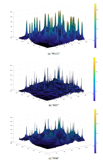Figure 18: Visual aspect of ML optimized WLC2 coverage when dim = 256

Conflict of Interest

The authors declare no conflict of interest.

Acknowledgment

We would thank colleagues researchers, engineers, and reviewers for sharing their precious comments and on-field experience that improved the quality of this paper.

1. M. Guessous and L. Zenkouar. “ML-Optimized Beam-based Radio Coverage Processing in IEEE 802.11 WLAN Networks”. In: 2018 5th International Conference on Electrical Engineering, Computer Science and Informatics (EECSI). Oct. 2018, pp. 564– 570. doi: 10.1109/EECSI.2018.8752874.
2.  Rafiza Ruslan and Tat-Chee Wan. “Cognitive radio-based power adjustment for Wi-Fi”. In: TENCON 2009-2009 IEEE Region 10 Conference. IEEE. 2009, pp. 1–5. doi: 10 . 1109 / TENCON.2009.5396078.
3. Daji Qiao et al. “Adaptive transmit power control in IEEE 802.11 a wireless LANs”. In: The 57th IEEE Semiannual Vehic- ular Technology Conference, 2003. VTC 2003-Spring. Vol. 1. IEEE. 2003, pp. 433–437. doi: 10 . 1109 / VETECS . 2003 . 1207577.
4. Nabeel Ahmed and Srinivasan Keshav. “A successive refine- ment approach to wireless infrastructure network deployment”. In: IEEE Wireless Communications and Networking Con-ference, 2006. WCNC 2006. Vol. 1. IEEE. 2006, pp. 511–519.
5.  Mehdi Guessous and Lahbib Zenkouar. “Cognitive direc- tional cost-based transmit power control in IEEE 802.11 WLAN”. In: 2017 International Conference on Information Net- working (ICOIN). IEEE. 2017, pp. 281–287. doi: 10 .1109 / ICOIN.2017.7899520.
6.  Prateek R Kapadia and Om P Damani. “Interference- constrained wireless coverage in a protocol model”. In: Pro- ceedings of the 9th ACM international symposium on Modeling analysis and simulation of wireless and mobile systems. ACM. 2006, pp. 207–211. doi: 10.1145/1164717.1164754.
7. Amit P Jardosh et al. “Green WLANs: on-demand WLAN infrastructures”. In: Mobile Networks and Applications 14.6 (2009), pp. 798–814. doi: 10.1007/s11036-008-0123-8.
8. Aditya Akella et al. “Self-management in chaotic wireless deployments”. In: Wireless Networks 13.6 (2007), pp. 737–755. doi: 10.1007/s11276-006-9852-4.
9.  Cem U Saraydar, Narayan B Mandayam, David J Goodman, et al. “Efficient power control via pricing in wireless data net- works”. In: IEEE transactions on Communications 50.2 (2002), pp. 291–303. doi: 10.1109/26.983324.
10. Dipankar Raychaudhuri and Xiangpeng Jing. “A spectrum etiquette protocol for efficient coordination of radio devices in unlicensed bands”. In: 14th IEEE Proceedings on Personal, Indoor and Mobile Radio Communications, 2003. PIMRC 2003.Vol. 1. IEEE. 2003, pp. 172–176. doi: 10.1109/PIMRC.2003.1264255.
11.  Radio Resource Management White Paper – Transmit Power Con- trol (TPC) Algorithm [Cisco 5500 Series Wireless Controllers]. en. June 2016. url: https :/ / www . cisco . com / c / en / us / td/docs/wireless/controller/technotes/8- 3/b_RRM_ White _ Paper / b _ RRM _ White _ Paper _ chapter _ 0101 .html (visited on 05/14/2019).
12.  ARM Coverage and Interference Metrics. url: https://www. arubanetworks . com / techdocs / ArubaOS _ 64x _ WebHelp / Content / ArubaFrameStyles / ARM / ARM _ Metrics . htm (vis- ited on 05/17/2019).
13.  Lowering the power level to reduce RF interference. url: https:/ / help . fortinet . com / fos50hlp / 52data / Content / FortiOS / fortigate – best – practices – 52 / Wireless / Lowering_Power_Level.htm (visited on 05/17/2019).
14.  Thomas M. Mitchell. Machine Learning. 1st ed. New York, NY, USA: McGraw-Hill, Inc., 1997. isbn: 0070428077, 9780070428072.
15. Mehdi Guessous and Lahbib Zenkouar. “A nurbs based technique for an optimized transmit opportunity map pro- cessing in wlan networks”. In: International Conference on Wired/Wireless Internet Communication. Springer. 2017, pp. 143–154. doi: 10.1007/978-3-319-61382-6_12.
16.  Alireza Babaei. “Longitudinal vibration responses of axi- ally functionally graded optimized MEMS gyroscope using Rayleigh–Ritz method, determination of discernible patterns and chaotic regimes”. In: SN Applied Sciences 1.8 (2019), 831. doi: 10.1007/s42452-019-0867-8.

(Click Here)

(Click Here)