
EKMC: Ensemble of kNN using MetaCost for Efficient Anomaly Detection
Volume 4, Issue 5, Page No 401-408, 2019
Author’s Name: Niranjan A1,a), Akshobhya K M1, P Deepa Shenoy1, Venugopal K R2
View Affiliations
1Department of Computer Science and Engineering, University Visvesvaraya College of Engineering, Bangalore University, Bangalore, India.
2Bangalore University, Bangalore, India.
a)Author to whom correspondence should be addressed. E-mail: a.niranjansharma@gmail.com
Adv. Sci. Technol. Eng. Syst. J. 4(5), 401-408 (2019); ![]() DOI: 10.25046/aj040552
DOI: 10.25046/aj040552
Keywords: Anomaly Detection, kNN, MetaCost

Export Citations
Anomaly detection aims at identification of suspicious items, observations or events by differing from most of the data. Intrusion Detection, Fault Detection, and Fraud Detection are some of the various applications of Anomaly Detection. The Machine learning classifier algorithms used in these applications would greatly affect the overall efficiency. This work is an extension of our previous work ERCRTV: Ensemble of Random Committee and Random Tree for Efficient Anomaly Classification using Voting. In the current work, we propose SDMR a simple Feature Selection Technique to select significant features from the data set. Furthermore, to reduce the dimensionality, we use PCA in the pre-processing stage. The EKMC (Ensemble of kNN using MetaCost) with ten-fold cross validation is then applied on the pre-processed data. The performance of EKMC is evaluated on UNSW_NB15 and NSL KDD data sets. The results of EKMC indicate better detection rate and prediction accuracy with a lesser error rate than other existing methods.
Received: 31 May 2019, Accepted: 29 September 2019, Published Online: 28 October 2019
1. Introduction
A process involving the identification of data points that do not fit with the remaining data points is referred to as Anomaly Detection. Hence, Anomaly Detection is employed by various machine learning applications involving the Detection of Intrusions, or Faults, and Frauds. Anomaly Detection can be achieved based either on nature of data or circumstances. There are three approaches for Anomaly Detection used under different circumstances: Static Rules approach, when the Training data is missing and when the Training data is available.
1.1. Static Rules Approach
In this approach, a list of known anomalies is identified, and rules are written to identify these anomalies. Rules are generally written using pattern mining techniques. Since identification of Static Rules is complex, machine learning approach that involves automatic learning of the rules is preferred.
1.2. When Training Data is missing
When the data set lacks a class label, we may use Unsupervised or Semi supervised learning techniques for Anomaly Detection. However, evaluating the performance of this approach is not possible because there shall be no test data either.
1.3. When Training Data is available
Even while the training set is available, the number of Anomaly samples will be too less when compared to the benign samples and hence there shall be class imbalance in such data sets. To overcome this problem, new sets are created by resampling data several times.
Anomaly detection can happen only after a successful classification. The efficiency of Anomaly Detection applications therefore depends on the classifiers used. Prediction Accuracy, ROC Area and Build time are some of such metrics that can measure the efficiency of a classifier. They are in turn based on Detection Rate (DR) and False Positive Rate (FPR). While DR is the correctness measure, FPR is the incorrectness measure during classification. ROC(Receiver Operating Characteristic) is a graphical representation of the ability of a binary classifier system obtained by varying its threshold. ROC involves plotting of TPR values (Y-axis) against FPR values (X-axis) at different threshold values. The time taken to train the given model is its build time. Any work is expected to have maximum value for DR and least or nil values for FPR, Error rates and Build time. This work focuses on the selection of features that are significant, from the data sets and reduction in their dimensionality while maintaining the detection accuracy. To achieve this, classifier algorithms with better individual performances are determined and are experimented with various combinations (ensemble) of classifiers. It was observed through our experiments that kNN offers best results in terms of the chosen metrics.
kNN is a typical classifier that learns based on instances. It is often referred to as a Lazy learning algorithm, because it defers computation until actual classification. The kNN algorithm assumes that similar things exist in proximity and therefore a sample from the test set is classified based on the predictions made by most of its neighbors.
Bagging, Boosting, Voting and Stacking are the ensembling techniques available today. The Bagging approach draws n instances randomly from a training set using a distribution that is uniform and learns them. The process is repeated several times. Every repetition generates one classifier. Boosting, a similar approach as that of bagging, focuses more on instances that were learnt incorrectly and monitors the performance of the machine learning algorithm. After constructing several classifiers in this manner, it performs a vote of the weights associated with the individual classifiers for making the final prediction. Each classifier is assigned weights based on its achieved detection accuracy on its training set. Voting requires the creation of several sub-models, allowing each of them to vote on the outcome of prediction. Stacking involves the training of different learning algorithms on the available data and providing the predictions of each learning algorithm as additional inputs to the combiner algorithm for the final training. In StackingC, Linear Regression is used as the Meta Classifier. A way of representing a linear equation by merging a set of input values (x) that are numeric into a predicted output value (y), may be defined as Linear Regression. This work involves an ensembling technique for the classification of the test samples present in the data set using MetaCost. MetaCost would produce results that are like the one that is created by passing the base learner (kNN in our case) to Bagging, which eventually is passed to a Cost Sensitive Classifier that operates on least expected cost. The only difference that we can observe is that MetaCost generates only one cost-sensitive classifier of the base learner, offering fast classification and interpretable output. This implementation uses all iterations of Bagging by reclassifying the training data.
Our experiments on the two benchmark data sets namely NSL-KDD and UNSW_NB15, prove that an ensemble of kNN using MetaCost yields better results compared to various machine learning algorithms. The NSL-KDD data set comprises of 41 features, and a class label to indicate an instance as normal or anomalous. The UNSW_NB15 data set on the other hand has 44 features plus one class label.
In this extension work [1], we propose SDMR for Feature Selection that exploits the advantages of various existing Weight Based Ranking Algorithms. In addition to SDMR, the data set is also subjected to PCA for dimensionality reduction during the preprocessing stage. The Principal Component Analysis (PCA) when applied on a data set having many variables (features) correlated with one another, reduces its dimensionality by only retaining the variation present in it. The existing variables of the data set are transformed to a new set of variables, known as the principal components (or PCs) that are orthogonal such that the correlation between any pair of variables is 0. The resultant set is then subjected to EKMC (Ensemble of kNN using MetaCost) with a cross validation of ten-folds before recording the performance metrics.
The details of our proposed framework are provided in Sections 3 and 4, respectively.
The key contributions of this extended paper are as follows.
1. SDMR (Standard Deviation of Mean of Ranks) to discard all those features whose ranks are less than the computed value,
- Use of PCA for the further reduction of dimensionality of the data set.
- EKMC Framework for efficient Anomaly classification.
The remainder of this article is organized as follows: Background and previous work related to ADS and our novel EKMC technique are explained in Section 3. Section 3 also discusses about the details of the novel SDMR Feature Selection technique. Section 4 presents the experimental results and analysis of the proposed EKMC using the two benchmark data sets. Finally, we conclude our work and suggest directions for further research.
2. Background and Related Works
ERCRTV [1] that forms the base work for the current work, uses Correlation based Feature Selection (CFS) algorithm for Feature Selection from the NSL KDD and KDD CUP 99 data sets. It selects only eight prominent features from them. The data subset with only chosen features is provided to an ensembled model of Random Committee and Random Forest using Voting. A ten-fold cross validation is performed on the model before recording the performance metrics. CFS being one of the Filter based Feature Selection algorithms, is faster, but is less accurate. Hence our current work involves a simple and more efficient SDMR technique for Feature Selection and Metacost classifier with kNN as the base classifier for the classification of Anomalous and benign samples. The MetaCost classifier relabels the class feature of the training set using meta learning technique. The modified training set is then used to produce the final model.
The authors of [2], propose a novel approach involving Two-layer dimensionality reduction followed by a Two-Tier classification for efficient detection of intrusions in IoT Backbone Networks. Their approach addresses the limitations of making wrong decisions and increased computational complexity of the classifier due to higher dimensionality. Component Analysis and Linear Discriminate Analysis form the Two Layers of Dimensionality Reduction during the preprocessing stage while Naïve Bayes and Certainty Factor variation of the K-Nearest Neighbor techniques form the Two Tiers of classification. A Detection Accuracy of 84.82 on twenty percent of the NSL-KDD training set is achieved by their work.
The methodology presented in [3] illustrates a detection technique based on anomaly detection involving data mining techniques. The paper discusses about the possible use of Apache Hadoop for parallel processing of extremely huge data sets. Dynamic Rule Creation technique that is adopted by their authors ensures that even new types of security breaches are detected automatically. The error rates of below ten percent can be observed from their findings.
The authors in their work [4], present a PSO-based feature selection followed by a two-tier ensembling model involving Boosting and Random Subspace Model (RSM). They illustrate with their results that accuracy and false positive rate (FPR) are better compared to all other models.
The work presented in [5] illustrates the importance of outlier detection in the training set that is achieved through Robust Regression technique during the preprocessing stage. Their work further proves that their model is far more superior to the normal Linear Regression technique that is used by most researchers. With their experimental data, the authors compare their model with Linear Regression Model and demonstrate that their Model is much superior especially in environments with bursty network traffic and pervasive network attacks.
The authors of [6] outline a Proactive Anomaly Detection Ensemble (ADE) technique for the timely anticipation of anomaly patterns in a given data set. Weighted Anomaly window is used as the ground truth to train the model allowing it to discover an anomaly well before its occurrence. They explore various strategies for the generation of ground truth windows. With their results, they establish that ADE exhibits at least ten percent improvement in earliest detection score as compared with other individual techniques across all the data sets that are considered for experimentation.
3. EKMC Technique
The current work revolves around Preprocessing and Classification phases. Feature Selection forms the main layer of preprocessing, since not all attributes in the data set are relevant during the analysis. We propose a novel SDMR for Feature Selection that exploits the advantages of various existing Weight Based Ranking Algorithms. In addition to SDMR, the data set is also subjected to PCA for dimensionality reduction during this phase. In the classification phase, we subject the resultant subset to the proposed EKMC algorithm with ten-fold cross validation for measuring the performance metrics. The framework of our proposed technique is depicted in Fig.1. The experiments are carried out on two benchmark data sets namely UNSW-NB15 and NSL-KDD. The NSL-KDD comprises of 125973 samples in the training and 22544 in the test set. EKMC model was trained making use of the training set and was then tested with the test set. The performance of the proposed model was further validated by running the model on UNSW-NB15 data set comprising of 175,341 records in the training set and 82,332 records in the test set.
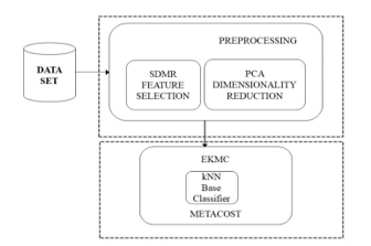 Figure 1: Proposed framework for Anomaly Detection
The various Weight based Feature Selection Algorithms that were employed to compute the Ranks Ri in the proposed SDMR are Information Gain, Information Gain Ratio, Weight by Correlation, Weight by Chi Squared Statistics, Gini Index, Weight by Tree importance, and Weight by Uncertainty. The SDMR that we obtained for the NSL KDD Data set was 0.278831 and that of UNSW-NB15 was 0.184325. All those features that are less than the SDMR values were discarded from the data sets. The proposed SDMR returned only 15 features out of 41 in case of NSL KDD and 11 features out of 44 features in case of UNSW-NB15. These subsets of features of both the data sets are further subjected to PCA for dimensionality reduction. The resulting feature subsets are finally subjected to the proposed EKMC framework. The proposed EKMC algorithm for efficient Anomaly Detection is presented in Algorithm 2. Table 1 and Table 2 list the Ranks determined using different Rank-Based Feature Selection Algorithms on NSL KDD and UNSW-NB 15 respectively. The proposed SDMR[7] for Feature Selection is presented in Algorithm1. The experimental results as indicated in Table 4 suggest that the kNN classifier offers best prediction accuracy, precision, recall, F-1 measure and Detection Accuracy with least classification error value out of the 20 classifier algorithms.
Algorithm 1: SDMR (Standard Deviation of Mean of Ranks) Feature Selection
Input: D data set having n number of Features
Output: subset F of D with Most Significant Features
- for each feature fi є D do
Determine Ranks Ri using different Weight Based Feature Selection Techniques
next
- for each feature fi є D do
Compute Sum (∑ Ri) and Mean mRi of Ranks
∑Ri = R1+ R2+ … + Rn and mRi =
next
- Compute Standard Deviation of Mean of Ranks SDMR
- Discard all fi є D < SDMR
- return F
Table 1: Feature Ranks of NSL KDD
| Attribute | Information Gain | Information gain ratio | Correlation | Chi Squared statistics | Gini Index | Tree importance | Uncertainty |
| f1_duration | 0.03 | 0.18 | 0.06 | 0.01 | 0.03 | 0.00 | 0.02 |
| f2_protocol_type | 0.09 | 0.12 | 0.07 | 0.11 | 0.11 | 0.00 | 0.16 |
| f3_service | 1.00 | 0.29 | 0.43 | 1.00 | 1.00 | 0.00 | 0.67 |
| f4_flag | 0.77 | 0.56 | 0.64 | 0.81 | 0.81 | 0.00 | 1.00 |
| f5_src_bytes | 0.90 | 1.00 | 0.01 | 0.00 | 0.96 | 1.00 | 0.00 |
| f6_dst_bytes | 0.85 | 0.94 | 0.00 | 0.00 | 0.89 | 0.94 | 0.00 |
| f7_land | 0.00 | 0.02 | 0.01 | 0.00 | 0.00 | 0.00 | 0.00 |
| f8_wrong_fragment | 0.01 | 0.22 | 0.13 | 0.01 | 0.01 | 0.00 | 0.04 |
| f9_urgent | 0.00 | 0.08 | 0.00 | 0.00 | 0.00 | 0.00 | 0.00 |
| f10_hot | 0.00 | 0.14 | 0.02 | 0.00 | 0.00 | 0.00 | 0.00 |
| f11_num_failed_logins | 0.00 | 0.10 | 0.00 | 0.00 | 0.00 | 0.00 | 0.00 |
| f12_logged_in | 0.60 | 0.69 | 0.92 | 0.64 | 0.64 | 0.00 | 1.00 |
| f13_num_compromised | 0.00 | 0.12 | 0.01 | 0.00 | 0.00 | 0.00 | 0.00 |
| f14_root_shell | 0.00 | 0.04 | 0.03 | 0.00 | 0.00 | 0.00 | 0.00 |
| f15_su_attempted | 0.00 | 0.12 | 0.03 | 0.00 | 0.00 | 0.00 | 0.00 |
| f16_num_root | 0.01 | 0.13 | 0.01 | 0.00 | 0.01 | 0.00 | 0.00 |
| f17_num_file_creations | 0.00 | 0.11 | 0.03 | 0.00 | 0.00 | 0.00 | 0.00 |
| f18_num_shells | 0.00 | 0.04 | 0.01 | 0.00 | 0.00 | 0.00 | 0.00 |
| f19_num_access_files | 0.00 | 0.12 | 0.05 | 0.00 | 0.00 | 0.00 | 0.01 |
| f20_num_outbound_cmds | 0.00 | 0.00 | 0.00 | 0.00 | 0.00 | 0.00 | 0.00 |
| f21_is_host_login | 0.00 | 0.08 | 0.00 | 0.00 | 0.00 | 0.00 | 0.00 |
| f22_is_guest_login | 0.00 | 0.03 | 0.05 | 0.00 | 0.00 | 0.00 | 0.01 |
| f23_count | 0.49 | 0.56 | 0.77 | 0.58 | 0.57 | 0.00 | 0.56 |
| f24_srv_count | 0.03 | 0.22 | 0.00 | 0.06 | 0.03 | 0.10 | 0.12 |
| f25_serror_rate | 0.55 | 0.72 | 0.87 | 0.58 | 0.58 | 0.00 | 0.91 |
| f26_srv_serror_rate | 0.56 | 0.72 | 0.86 | 0.58 | 0.58 | 0.68 | 0.93 |
| f27_rerror_rate | 0.08 | 0.15 | 0.34 | 0.09 | 0.09 | 0.00 | 0.15 |
| f28_srv_rerror_rate | 0.07 | 0.16 | 0.34 | 0.09 | 0.09 | 0.00 | 0.15 |
| f29_same_srv_rate | 0.70 | 0.82 | 1.00 | 0.77 | 0.75 | 0.79 | 0.94 |
| f30_diff_srv_rate | 0.67 | 0.77 | 0.27 | 0.03 | 0.74 | 0.73 | 0.06 |
| f31_srv_diff_host_rate | 0.14 | 0.21 | 0.16 | 0.12 | 0.16 | 0.00 | 0.19 |
| f32_dst_host_count | 0.22 | 0.26 | 0.50 | 0.27 | 0.27 | 0.00 | 0.25 |
| f33_dst_host_srv_count | 0.59 | 0.66 | 0.96 | 0.74 | 0.67 | 0.60 | 0.71 |
| f34_dst_host_same_srv_rate | 0.59 | 0.66 | 0.92 | 0.71 | 0.67 | 0.00 | 0.69 |
| f35_dst_host_diff_srv_rate | 0.51 | 0.57 | 0.32 | 0.71 | 0.59 | 0.49 | 0.06 |
| f36_dst_host_same_src_port_rate | 0.14 | 0.16 | 0.12 | 0.06 | 0.17 | 0.00 | 0.07 |
| f37_dst_host_srv_diff_host_rate | 0.22 | 0.28 | 0.08 | 0.04 | 0.26 | 0.00 | 0.09 |
| f38_dst_host_serror_rate | 0.56 | 0.74 | 0.87 | 0.59 | 0.57 | 0.70 | 0.91 |
| f39_dst_host_srv_serror_rate | 0.58 | 0.76 | 0.87 | 0.58 | 0.58 | 0.00 | 0.97 |
| f40_dst_host_rerror_rate | 0.07 | 0.14 | 0.34 | 0.09 | 0.09 | 0.00 | 0.13 |
| f41_dst_host_srv_rerror_rate | 0.11 | 0.25 | 0.34 | 0.11 | 0.12 | 0.00 | 0.19 |
Table 2: Feature Ranks of UNSW-NB 15
| Attribute | Information Gain | Information gain ratio | Correlation | Chi Squared statistics | Gini index | Tree importance | Uncertainty |
| f1_id | 0.32 | 0.51 | 0.49 | 0.62 | 0.38 | 0.83 | 0.46 |
| f2_dur | 0.20 | 0.29 | 0.04 | 0.00 | 0.24 | 0.13 | 0.01 |
| f3_proto | 0.19 | 0.08 | 0.33 | 0.20 | 0.20 | 0.00 | 0.20 |
| f4_service | 0.08 | 0.00 | 0.28 | 0.09 | 0.09 | 0.00 | 0.10 |
| f5_state | 0.27 | 0.27 | 0.65 | 0.32 | 0.32 | 0.30 | 0.39 |
| f6_spkts | 0.11 | 0.16 | 0.05 | 0.00 | 0.14 | 0.30 | 0.00 |
| f7_dpkts | 0.20 | 0.30 | 0.12 | 0.00 | 0.25 | 0.07 | 0.00 |
| f8_sbytes | 0.11 | 0.30 | 0.02 | 0.00 | 0.14 | 1.00 | 0.00 |
| f9_dbytes | 0.20 | 0.30 | 0.08 | 0.00 | 0.25 | 0.03 | 0.00 |
| f10_rate | 0.24 | 0.37 | 0.43 | 0.25 | 0.27 | 0.24 | 0.29 |
| f11_sttl | 0.46 | 1.00 | 0.80 | 0.54 | 0.53 | 0.90 | 0.70 |
| f12_dttl | 0.20 | 0.29 | 0.02 | 0.52 | 0.24 | 0.48 | 0.63 |
| f13_sload | 0.24 | 0.38 | 0.21 | 0.00 | 0.28 | 0.15 | 0.00 |
| f14_dload | 0.26 | 0.58 | 0.45 | 0.13 | 0.33 | 0.25 | 0.26 |
| f15_sloss | 0.10 | 0.14 | 0.00 | 0.00 | 0.13 | 0.19 | 0.00 |
| f16_dloss | 0.10 | 0.21 | 0.10 | 0.00 | 0.14 | 0.08 | 0.00 |
| f17_sinpkt | 0.13 | 0.30 | 0.20 | 0.02 | 0.17 | 0.08 | 0.07 |
| f18_dinpkt | 0.20 | 0.30 | 0.04 | 0.00 | 0.24 | 0.02 | 0.00 |
| f19_sjit | 0.10 | 0.11 | 0.02 | 0.00 | 0.13 | 0.11 | 0.00 |
| f20_djit | 0.10 | 0.10 | 0.06 | 0.00 | 0.13 | 0.10 | 0.00 |
| f21_swin | 0.10 | 0.11 | 0.47 | 0.13 | 0.13 | 0.00 | 0.18 |
| f22_stcpb | 0.09 | 0.09 | 0.34 | 0.10 | 0.12 | 0.00 | 0.08 |
| f23_dtcpb | 0.09 | 0.09 | 0.34 | 0.09 | 0.12 | 0.00 | 0.07 |
| f24_dwin | 0.09 | 0.09 | 0.43 | 0.12 | 0.12 | 0.00 | 0.16 |
| f25_tcprtt | 0.09 | 0.17 | 0.03 | 0.01 | 0.11 | 0.06 | 0.02 |
| f26_synack | 0.09 | 0.16 | 0.05 | 0.00 | 0.11 | 0.21 | 0.01 |
| f27_ackdat | 0.09 | 0.16 | 0.00 | 0.00 | 0.11 | 0.13 | 0.01 |
| f28_smean | 0.05 | 0.05 | 0.04 | 0.02 | 0.06 | 0.29 | 0.02 |
| f29_dmean | 0.20 | 0.30 | 0.38 | 0.10 | 0.25 | 0.09 | 0.12 |
| f30_trans_depth | 0.00 | 0.00 | 0.00 | 0.00 | 0.00 | 0.12 | 0.00 |
| f31_response_body_len | 0.01 | 0.10 | 0.02 | 0.00 | 0.01 | 0.00 | 0.00 |
| f32_ct_srv_src | 0.08 | 0.13 | 0.31 | 0.09 | 0.09 | 0.14 | 0.11 |
| f33_ct_state_ttl | 0.41 | 0.90 | 0.61 | 0.56 | 0.48 | 0.40 | 0.62 |
| f34_ct_dst_ltm | 0.09 | 0.17 | 0.31 | 0.09 | 0.09 | 0.09 | 0.13 |
| f35_ct_src_dport_ltm | 0.11 | 0.22 | 0.41 | 0.12 | 0.12 | 0.02 | 0.19 |
| f36_ct_dst_sport_ltm | 0.21 | 0.37 | 0.47 | 0.14 | 0.20 | 0.12 | 0.26 |
| f37_ct_dst_src_ltm | 0.10 | 0.16 | 0.38 | 0.11 | 0.11 | 0.12 | 0.14 |
| f38_is_ftp_login | 0.00 | 0.00 | 0.01 | 0.00 | 0.00 | 0.00 | 0.00 |
| f39_ct_ftp_cmd | 0.00 | 0.00 | 0.01 | 0.00 | 0.00 | 0.00 | 0.00 |
| f40_ct_flw_http_mthd | 0.00 | 0.01 | 0.01 | 0.00 | 0.00 | 0.00 | 0.00 |
| f41_ct_src_ltm | 0.09 | 0.16 | 0.32 | 0.09 | 0.09 | 0.00 | 0.12 |
| f42_ct_srv_dst | 0.08 | 0.14 | 0.32 | 0.10 | 0.09 | 0.13 | 0.11 |
| f43_is_sm_ips_ports | 0.02 | 0.31 | 0.20 | 0.03 | 0.03 | 0.15 | 0.07 |
| f44_attack_cat | 1.00 | 0.68 | 1.00 | 1.00 | 1.00 | 0.73 | 1.00 |
Algorithm 2: Ensemble of kNN using MetaCost (EKMC)
Input: subset F after applying PCA
Output: Performance Metrics
- Subject input to an Ensemble of MetaCost with kNN Base Classifier.
- Perform cross validation of ten-folds and record the performance metrics.
Encouraged by the results of kNN, we tried ensembling kNN using Bagging, Classification by Regression and MetaCost and the results as indicated in Table 4 prove that MetaCost happens to be the most efficient of them all.
4. Experimental Results and Discussion
The experiments are carried out on two benchmark data sets UNSW-NB15 and NSL-KDD. The NSL-KDD has 125973 instances in the training and 22544 instances in the test set. EKMC was trained using the training set and was tested making use of the test set. Performance metrics after a more rigorous ten-fold cross validation were then recorded. The performance of the proposed model was later validated using the UNSW-NB15. The UNSW-NB15 comprises of 175,341 instances in the training set and 82,332 instances in the test set. A ten-fold cross validation typically involves dividing the input data set into ten parts and training the model with the nine parts while using the excluded part as the test set and repeating the process for a total of ten times by using an unused test set during each round.
The SDMR Feature Selection algorithm as listed in Algorithm 1 involves the computation of ranks for each feature. Information Gain, Information Gain Ratio, Weight by Correlation, Weight by Chi Squared Statistics, Gini Index, Weight by Tree importance, and Weight by Uncertainty are used for the computation of Ranks. The weights of each feature of NSL KDD data set are listed in Table 1 and that of UNSW-NB 15 in Table 2. The mean value of Weights of Ranks of each Feature as determined by all the chosen Algorithms is initially determined. A Standard Deviation of Mean of Ranks is then Computed. All those Features whose Mean of Ranks is less than or equal to the computed SDMR are dropped and only the Features whose Mean of Ranks is greater than the SDMR are selected. The SDMR of NSL KDD is found to be 0.278831 and that of UNSW-NB 15 is 0.184325. After dropping the Features whose Mean of Ranks is less than the SDMR value, only 15 Features from the NSL-KDD and 11 Features from the UNSW-NB data set are selected.
In addition to SDMR, the data set is also subjected to PCA for dimensionality reduction during the preprocessing stage. The Principal Component Analysis (PCA) when applied on a data set having many variables (features) correlated with one another, reduces its dimensionality by only retaining the variation present in it. The existing variables of the data set are transformed to a new set of variables, known as the principal components (or PCs) that are orthogonal such that the correlation between any pair of variables is 0.The resultant set is subjected to various built-in Classifier Algorithms with ten-fold cross validation to measure the performance metrics. The performance of the Classifier Algorithms is evaluated based on the Accuracy, Classification Error, Precision, Recall, F1-Measure and Detection Rates.
Efficiency of classification would be better when a classifier exhibits true positive rates that are maximum and false positive rates that are minimum. In this context, 8 Performance metrics of classification process are defined. Let Nben represent total number of normal or benign samples and Nanom the number of anomalous samples in a data set. True Positive (TP) is the number of normal or benign instances classified correctly as normal is denoted as Nbenàben and True Negative (TN) is the number of anomalous instances classified correctly as anomalous is denoted as Nanomàanom. False Positive (FP) is a measure of normal instances misclassified as anomalous is denoted as Nbenàanom while False Negative (FN) is a measure of anomalous instances misclassified as normal is denoted as Nanomàben.
The Detection Rate (DR) is the rate of anomalous samples being classified correctly as anomalous.
TPR= X 100 (1)
False positive rate (FPR) is the rate of normal samples being classified incorrectly as anomalous samples.
FPR = X 100 (2)
False Negative Rate (FNR) is the rate of anomalous samples being classified incorrectly as benign samples.
FNR = X 100 (3)
True Negative Rate (TNR) is the rate of benign samples being classified correctly as benign out of the total available benign samples.
TNR = X100 (4)
Prediction Accuracy (PA) is the total number of anomalous and benign samples that are identified correctly with respect to the total number of all available samples.
PA = X 100 (5)
Precision is the number of true positives divided by the total number of elements labeled as belonging to the positive class.
Precision = X100 (6)
Recall is the number of true positives divided by the total number of elements that really belong to the positive class.
Recall = X 100 (7)
F1-Measure is the harmonic mean of Precision and Recall and is given by:
F1-Measure= (8)
The experimental results as indicated in Table 3 suggest that the kNN classifier offers best Prediction Accuracy, Precision, Recall, F-1 measure and Detection Accuracy with least classification error value out of the 20 classifier algorithms. This prompted us to use kNN as the Base Classifier in the Ensembled approach. When different Ensembling Schemes such as Bagging, Classification by Regression and MetaCost were used, only MetaCost with kNN as the Base Classifier offered best results in comparison with the other two approaches as indicated in Table 4 and plotted on a graph as depicted in Figure 3. This was the reason behind choosing MetaCost with kNN as the Base Classifier in our proposed work.
The proposed EKMC performs better than our previous model i.e. ERCRTV [1] and the existing GAA-ADS [8] models when tested on both the data sets. EKMC exhibits good Prediction Accuracy and a better Detection Rate as listed in Table 5 and depicted in Figure 2.
Table 3: Classification result
| Classification Algorithm | Accuracy | Classification Error | Precision | Recall | F1 Measure | Detection rate |
| Perceptron | 49.37% | 50.63% | 68.08% | 2.88% | 5.26% | 2.88% |
| Neural Net | 50.75% | 49.25% | 48.12% | 30.00% | 36.96% | 30.00% |
| Quadratic Discriminant Analysis | 51.29% | 48.71% | 4.57% | 0.06% | 0.12% | 0.06% |
| Regularized Discriminant Model | 51.63% | 48.37% | 8.01% | 0.05% | 0.10% | 0.05% |
| Naïve Bayes | 51.71% | 48.29% | 21.10% | 0.13% | 0.26% | 0.13% |
| CHAID | 51.88% | 48.12% | unknown | 0.00% | unknown | 0.00% |
| Default Model | 51.88% | 48.12% | unknown | 0.00% | unknown | 0.00% |
| Generalised Linear Model | 51.89% | 48.11% | 90.91% | 0.01% | 0.03% | 0.01% |
| Linear Discriminant Model | 51.89% | 48.11% | 90.91% | 0.01% | 0.03% | 0.01% |
| Linear Regression | 51.89% | 48.11% | 87.50% | 0.01% | 0.02% | 0.01% |
| Logistic Regression | 51.89% | 48.11% | 68.42% | 0.02% | 0.04% | 0.02% |
| Deep Learning | 52.71% | 47.29% | 53.91% | 88.42% | 60.83% | 88.42% |
| Naïve Bayes Kernel | 60.32% | 39.68% | 39.68% | 77.63% | 77.63% | 77.63% |
| Decision Stump | 90.35% | 9.65% | 92.36% | 87.15% | 89.68% | 87.15% |
| Gradient Boosted Tree | 93.54% | 6.46% | 91.85% | 95.09% | 93.42% | 95.09% |
| Random Tree | 94.24% | 5.76% | 92.90% | 95.31% | 94.09% | 95.31% |
| Rule Induction | 94.45% | 5.55% | 93.96% | 94.54% | 94.25% | 94.54% |
| Decision Tree | 95.54% | 4.46% | 94.36% | 96.51% | 95.42% | 96.51% |
| Random Forest | 95.74% | 4.26% | 94.67% | 96.58% | 95.62% | 96.58% |
| kNN | 98.85% | 1.15% | 98.88% | 98.73% | 98.81% | 98.73% |
Table 4: Comparison of Ensembling Techniques
| Ensembling Technique | Accuracy | Classification Error | Precision | Recall | F1 Measure | Detection rate |
| Bagging | 98.87% | 1.13% | 98.88% | 98.76% | 98.82% | 98.76% |
| Classification by Regression | 98.85% | 1.15% | 98.88% | 98.73% | 98.81% | 98.73% |
| Meta cost | 98.90% | 1.10% | 98.92% | 98.80% | 98.86% | 98.80% |
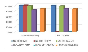 Figure 2: Comparison graph of Various available Models
Table 5: Performance Comparison of the techniques on NSL-KDD and UNSW-NB 15 data sets.
| Data set | Method | Accuracy | Detection Rate |
|
NSL KDD |
EKMC | 98.90% | 98.80% |
| ERCRTV[1] | 99.60% | 0 | |
| GAA-ADS[8] | 97.30% | 96.76% | |
|
UNSW NB15 |
EKMC | 81.58% | 87.60% |
| ERCRTV[1] | 0 | 0 | |
| GAA-ADS[8] | 87.46% | 86.04% |
5. Conclusion
In the Pre-processing phase[9,10], Feature Selection using SDMR is applied to select only significant features from the data set. The SDMR Feature Selection algorithm is very much novel and greatly reduces the dimensionality of the data set almost equaling to 70%. It selects only 15 features out of 41 features in case of NSL-KDD and a mere 11 features out of 44 features in case of UNSW-NB15. PCA is then applied to further reduce dimensionality of the data set. The proposed EKMC outperforms GAA-ADS in terms of Detection rate on both the data sets. The detection rates of EKMC are 98.8% and 87.60% on NSL-KDD and UNSW-NB15 respectively while that of GAA-ADS are 96.76 and 86.04% respectively on the same data sets. The performance metrics are recorded for tenfold cross validation. The proposed model is required to be tested on other data sets as well and Classification Error rate must further be reduced.
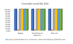 Figure 3: Comparison of Ensembling techniques graph
- A. Niranjan, D. H. Nutan, A. Nitish, P. D. Shenoy and K. R. Venugopal, “ERCR TV: Ensemble of Random Committee and Random Tree for Efficient Anomaly Classification Using Voting,” 2018 3rd International Conference for Convergence in Technology (I2CT), Pune, 2018, pp. 1-5.
- doi: 10.1109/I2CT.2018.8529797H Haddad Pajouh, R Javidan, R Khayami, D Ali and K K R Choo, “A Two-layer Dimension Reduction and Two-tier Classification Model for Anomaly-Based Intrusion Detection in IoT Backbone Networks”, IEEE Transactions on Emerging Topics in Computing, vol. pp, no. 99, pp. 1- 11.
- Jakub Breier and Jana Branisov,“Anomaly Detection from Log files using Data Mining Techniques”, Proceedings of Conference on Information Science and Applications (Springer), vol. 339, 2015, pp. 449-457.
- Bayu Adhi Tama, Akash Suresh Patil, Kyung-Hyune Rhee “An Improved Model of Anomaly Detection using Two-level Classifier Ensemble”, Proceedings of 12th Asia Joint Conference on Information Security, 2017.
- Ziyu Wang, Jiahai Yang, Zhang ShiZe, Chenxi Li “Robust Regression for Anomaly Detection”, Proceedings of IEEE ICC 2017 Communication and Information Systems Security Symposium, 2017.
- Teodora Sandra Buda1, Haytham Assem1 and Lei Xu1 “ADE: An Ensemble Approach for Early Anomaly Detection”, Integrated Network and Service Management (IM), 2017 IFIP/IEEE Symposium, 2017.
- A. Niranjan, K. M. Akshobhya, P. D. Shenoy and K. R. Venugopal, “EKNIS: Ensemble of KNN, Naïve Bayes Kernel and ID3 for Efficient Botnet Classification Using Stacking,” 2018 International Conference on Data Science and Engineering (ICDSE), Kochi, 2018, pp. 1-6.doi: 10.1109/ICDSE.2018.8527791
- N. Moustafa, J. Slay and G. Creech, “Novel Geometric Area Analysis Technique for Anomaly Detection using Trapezoidal Area Estimation on Large-Scale Networks,” in IEEE Transactions on Big Data. doi: 10.1109/TBDATA.2017.2715166
- Niranjan A, Nitish A, P Deepa Shenoy and Venugopal K R, “Security in Data Mining-a Comprehensive Survey”, Global Journal of Computer Science and Technology, vol. 16, no. 5, 2017, pp. 52-73.
- Asha S Manek, Samhitha M R, Shruthy S , Veena H Bhat, P Deepa Shenoy, M. Chandra Mohan, Venugopal K R, L M Patnaik “RePID-OK: Spam Detection using Repetitive Pre-processing”, IEEE CUBE 2013 Conference, ISBN : 978-1-4799-2234-5, pp. 144-149, November 15-16, 2013.