1. Introduction

Nowadays bitcoin has become the most popular cryptocurrency and has the largest capitalization value compared to others cryptocurrency. Besides being a digital currency, bitcoin has also become a trading instrument. The price of bitcoin has very high volatility. Even though it has high volatility and is full of risks and uncertainties, many people are interested in trading bitcoin. The high volatility of bitcoin price movements has encouraged many people to speculate on getting high capital gains. To assist bitcoin traders, a system that is capable to predict the price of bitcoin is needed, which intended to increase the potential to get large profits as well as to avoid potential losses

In recent years there have been many studies that use deep learning for predicting the price of bitcoin. Adebiyi et al. [1] and Guresen et al. [2] used Multi Layer Perceptron (MLP) while Jang and Lee [3] and McNally et al. [4] used Bayesian Neural Network. Deep learning model that is widely used for predicting bitcoin prices is Long Short-Term Memory Neural Network (LSTM) [4], [5]. LSTM is a special modification of Recurrent Neural Network (RNN). LSTM is widely used in time series forecasting activities because of its ability in remembering long sequential data.

The use of model that use LSTM for predicting bitcoin prices has a disadvantage, it requires a long training time [4] and a suitable hyperparameter combination is needed to get optimal results. There were several researches that tried to optimize hyperparameters in models that use LSTM using metaheuristics such as Particle Swarm Optimization (PSO) [6], Genetic Algorithm (GA) [7] and Ant Colony Optimization (ACO) [8]. The use of metaheuristic for optimizing hyperparameters on model that use LSTM was expected to get a model with small error.

In this research, a sliding window was conducted on the closing price of bitcoin and bitcoin volume traded from the previous days as a feature for price predictions of bitcoin in the next day. Using sliding window can improve the accuracy of bitcoin predictions [9]. To get the appropriate sliding window numbers, the sliding window was used as one of the optimized hyperparameter. This research used Artificial Bee Colony (ABC) as a method for optimizing hyperparameter for models that use LSTM for bitcoin price prediction.

ABC is a metaheuristic algorithm based on foraging behavior of bee colonies [10]. ABC had been used as an optimization algorithm in many task [11], such as training neural network [12]. Besides that ABC also used as a machine learning method, such as clustering [13]. ABC has a good balance in exploiting and exploring solution [14]. In this research ABC was proposed as an optimization method for optimizing hyperparameter.

The main contribution of this research is combining ABC and LSTM to optimize the hyperparameter that resulted a model with small RMSE. Optimized hyperparameter in this research consisted of sliding window size, number of LSTM units, dropout rate, regularizer, regularizer rate, optimizer and learning rate. Chung and Shin [7] combined GA and LSTM for optimizing hyperparameter consisted of sliding window size and number of LSTM units.

This paper is structured as follows. Section 2 contains the literature review, Section 3 contains the proposed method in this research, which is the combination of ABC and LSTM for optimizing hyperparameter, Section 4 contains an explanation of dataset, implementation, experiment results and comparison with benchmark models and Section 5 contains conclusion of this research.

2. Literature Review

2.1.  Related Works

An old model that is often used for forecasting is the Auto Regressive Integrated Moving Average (ARIMA). Saxena et al. [15] used ARIMA model and compared its performance with LSTM model for predicting bitcoin prices. Bitcoin price prediction using LSTM outperformed ARIMA [15]. Similar to stock prices, bitcoin prices is often nonlinear and non-stationary, thus the application of the ARIMA model for long-term predictions is quite difficult [16].

In recent years, there are many researches tried to predict price movement by using deep learning. Deep learning is basically Artificial Neural Network (ANN) with input layers, several hidden layers and output layers which are usually referred to as Multi Layer Perceptron (MLP). Adebiyi et al. [1] used ANN for predicting stock prices.

Guresen et al. [2] used MLP, Dynamic Artificial Neural Network (DAN2) and hybrid neural network by using a generalized autoregressive conditional heteroscedasticity (GARCH) for predicting a stock market index.

Bayesian Optimized Recurrent Neural Network was used by McNally et al. [4] for predicting the classification of bitcoin prices movement that slightly outperformed the ARIMA model. McNally et al. [4] also used LSTM model with accuracy that exceeded the Bayesian Optimized RNN but the time needed by LSTM for training data was much longer than Bayesian Optimized RNN. This LSTM model had been proven effective for predicting bitcoin prices [4]. Jang and Lee [3] also used Bayesian Neural Network for predicting bitcoin prices based on bitcoin time series data and other blockchain information.

A model that use LSTM was also used by Alessandretti et al. [5] for predicting the cryptocurrency market where LSTM performed better for predictions with longer data days than models that use Gradient Boosting Decision Tree. LSTM for predicting stock price movements used in  [17]–[19]. Nelson et al. [20] used LSTM to predict stock market price movements. Gao and Chai [19] used a stock prediction model that combines LSTM with PCA. Table 1 shows summary of related works. It describes dataset and method that was used and the experiment results.

Table 1: Summary of related works

Ref	Dataset	Method	Result
[15]	Bitcoin Price	LSTM	LSTM outperformed ARIMA
		ARIMA
[4]	Bitcoin Price	Bayesian Optimized RNN	LSTM achieved highest classification accuracy while RNN achieved lowest RMSE
		LSTM
		ARIMA
[5]	Bitcoin Price	Single Regression XGBoost	Regression XGBoost  worked best for short time window while LSTM worked best for long time window
		Multi Regression XGBoost
		LSTM
		Simple Moving Average
[9]	Bitcoin Price, prices of crude oil, SSE, gold, VIX, FTSE100, global currencies USD/CNY, USD/JPY, USD/CHF	Support Vector Regression	LSTM outperformed all other model
		Linear Regression
		Neural Network
		LSTM
[21]	Bitcoin Price	PSO-MLP-NARX	The model was able to predict accurately while passing all model validation tests

Huisu et al. [9] used the LSTM model rolling window in several input features and information about blockchain information. This model accurately predicted the price of bitcoin. LSTM was also used by Yunbeom and Hwang [22] by comparing its performance with several neural networks namely Deep Neural Network (DNN), basic RNN, RNN with LSTM cell, RNN with GRU cell and bidirectional RNN. Best performance in specifity, precision  and accuracy achieved by DNN while best performance in sensitivity achieved by Bidirectional RNN.

Some metaheuristic algorithms were used to optimize model that use LSTM such as Genetic Algorithm, Ant Colony Optimization and Particle Swarm Optimization [6]–[8]. Chung and Shin [7] used a model that use LSTM that is optimized using Genetic Algorithm (GA) for predicting the stock market. In metaheuristics, the trial and error method is usually used as the basis for estimation in determining the time window size and LSTM architecture to be used in the research model. In [7], a systematic method was used to determine the time window size and LSTM topology for predicting the stock market. In deep learning, it is very difficult to determine the optimal architectural parameters. [7] showed that the model can be used as an effective tool to determine the optimal or near optimal model in deep learning.

Chhachhiya et al. [6] designed architecture of a model that use LSTM by using Particle Swarm Optimization (PSO). This hybrid model optimizes 3 parameters, namely activation function, learning rate and hidden neurons. The parameter that produced the smallest RMSE value is the most optimal model.

Sheikhan and Mohammadi [23] used GA-ACO + PSO-MLP for predicting time series data. Sun et al. [24] combined AdaBoost-LSTM Ensemble Learning for conducting a financial time series Forecasting. Indera et al. [21] used MLP which was optimized by using PSO for predicting the price of bitcoin.

2.2.  Long Short Term Memory (LSTM)

LSTM is a type of Recurrent Neural Network (RNN) where modifications are made to the RNN architecture by adding a memory cell that can store information for a long period of time [25]. LSTM was proposed as a solution to overcome the vanishing gradient or exploding gradient problems that occur in RNN. This problem occurs when processing very long sequential data. This gradient problem caused RNN failing to capture long term dependencies [15]. Vanishing or exploding gradient problem will reduce the accuracy of a RNN model that affected the output of a prediction [26].

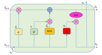Figure 1: Architecture of LSTM

In a LSTM cell there is a memory cell and 3 gates, namely the input gate, the forget gate and the output gate. Figure 1 shows the architecture of LSTM and the processing of input data. The process of LSTM is carried out in the following stages [7]:

1. The value of an input can only be stored in the cell state only if it is permitted by the input gate. Calculation of the values ​​at input gate and candidate inputs from the cell state is carried out using (1) and Eq. (2).

Where  is the value of input gate,  is the weight for the input value at time to t,  is the input value at time to t,  is the weight for the output value from time to t-1,  is the output value from time to t-1 and  is the bias at the gate input and σ is the sigmoid function.

Where  is the candidate cell state value,  is the weight for the input value in cell to c,  is the input value at time to t,  is the weight for the output value of cell to c-1,  is the value the output of cell to c-1 and  is bias in cell to c and tanh is a hyperbolic tangent function.

2. Then the forget gate value is calculated using (3).

Where  is the forget gate value,  is the weight for the input value at time to t,  is the input value at time to t,  is the weight for the output value from time to t-1,  is the output value from time to t-1 and  is the bias on the forget gate and σ is a sigmoid function.

3. Furthermore the cell state memory is calculated using (4).

Where  is the memory cell state value,  is the value of the gate input,  is the candidate memory cell state value,  is the forget gate value and  is the cell state memory value in the previous cell.

4. After generating a new cell state memory, the value of the gate output can be calculated using (5).

Where  is the value of the gate output,  is the weight for the input value at time to t,  is the input value at time to t,  is the weight for the output value from time to t-1,  is the output value from time to t-1 and  is the bias at the gate output and σ is the sigmoid function.

5. The final output value is calculated using (6).

Where  is the final output,  is the gate output value,  is the new memory cell state value and the tan is the hyperbolic tangent function.

2.3.  Artificial Bee Colony

Artificial Bee Colony algorithm was first proposed by Karaboga in 2005. It is a metaheuristic algorithm based on bee colonies. This algorithm mimics the intelligent behavior of bee colonies in foraging. In ABC, a colony of bees is divided into 3 types. Employee bee that is responsible for exploiting food sources, onlooker bee that is participating in exploiting food sources based on food information received from employee bee in waggle dance and scout bee that is tasked to find a new food source.

In ABC Algorithm, solutions of the optimization problem is described as a food source (nectar) [11]. And the quality of nectar describes the objective function of a solution. The number of food sources is the same as the number of employee bees, while the number of employee bees is the same as the number of onlooker bees. Bee behavior in foraging can be described as follows [11]:

1. At the initial stage of looking for food sources, bees start randomly exploring the area around the nest to get food sources.
2. After finding food sources, bees begin to become employee bees and start exploiting food sources found. After that. the employee bee will return to the nest by carrying nectar and unloading the nectar. After unloaded the nectar, the employee bee can immediately return to the food source or the bee can share information about the food source to other bees by doing Waggle Dance. The number of movements in dance shows the quality of nectar. If the nectar has run out, the employee bee will become a bee scout and start looking for other food sources randomly.
3. Onlooker bees waiting in the nest and choose the food source after watching waggle dance performed by employee

          Based on the behavior of bee colonies in foraging, the steps of the Artificial Bee Colony algorithm can be described as follows [12]:

1. Initialize the solution using (7). Each solution is a vector with D dimensions.

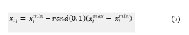      Where i = 1. . . SN, j = 1. . . D. SN is the number of food sources (solution) and D is the number of optimized hyperparameters.

2. Evaluate all solutions
3. Cycle = 1. The optimal parameter search process is in cycles, C = 1, 2. . . , MCN.
4. Repeat step 5 to 12 until cycle = Maximum Cycle Number (MCN)
5. Create a new solution for each employee bee from the  solution using (8) and evaluate the results. This new solution is a modification of the previous solution.

      Where k ∈ {1,2, …, SN) and j ∈ {1,2, …, D) are randomly selected indexes.

6. Perform the selection process. If the cost function of the new solution is smaller than the previous solution, the solution will be updated to the new solution. The employee’s bee will then remember the new, better solution.
7. Calculate the probability valuefor the  solution using (9) and Eq. (10).

      Where  is the value of the objective function solution i.

      Where  is the fitness value of the value of the objective function solution i. And SN is the number of solutions.

8. The onlooker bee evaluates the solution based on the information provided by the employee bee then selects which solution to follow based on the probability of calculated using (10). Create a new  solution for each onlooker bee from the solution selected based on the probability of  using Eq. (7) and evaluating the results. As with the bee employee, this solution is a modification of the selected  solution.
9. Perform the selection process. If the cost function of the new solution is smaller than the previous solution, the solution will be updated to the new solution. The employee bee will memorize the new
10. If there is a bee when modifying a solution does not get a new solution that is better than the previous solution until certain limit, then the solution will be abandoned, and the bee becomes a scout bee and randomly searches new food sources using (7). The new solution will replace the old solution that was abandoned.
11. Save the best solution up to now
12. Cycle = cycle + 1

3. Proposed Method

3.1.  The Concept

Optimized hyperparameter in this research consisted of sliding window size (h₁), number of LSTM units (h₂), dropout (h₃), regularizer (h₄), regularizer rate (h₅), optimizer (h₆) and learning rate (h₇). Each hyperparameter has a different range of values. The concept of optimizing hyperparameter in the model that use LSTM using ABC is to make these hyperparameters as dimension of problems, thus there are 7 dimensions of the problem. Each combination of the 7 dimensions of the problem is a solution that represents a model that use LSTM. Those solutions in the form of a combination of hyperparameters are described as genes in a chromosome in the genetic algorithm as can be seen in Figure 2. Those solutions will be trained and then predictions will be made. The prediction results of the model is measured using RMSE and considered as the fitness function of a solution on ABC.

Figure 2: dimension of hyperparameter (dimension of problem)

Next, those solutions will be optimized by changing one of the values ​​of the 7 dimensions of the hyperparameter randomly and then conducting training and prediction using the modified solutions. If the modified solution is better than previous solution, the solution will be updated. The process continues until the maximum cycle numbers specified in the ABC parameters setting is reached.

3.2.  Artificial Bee Colony – Long Short Term Memory (ABC-LSTM)

The hyperparameter optimization process on LSTM using the Artificial Bee Colony is carried out in following steps :

1. Randomly generate N initial solutions (food sources) using Eq. (7). In this case the solutions are hyperparameter combination for training LSTM.
2. Conducting LSTM training using the initial hyperparameter, evaluating and memorizing the lowest fitness function, in this case is the RMSE value of the prediction
3. Employee bee evaluates the RMSE produced by the initial solutions and tries to modify the hyperparameter combination to minimize RMSE using Eq. (8).
4. Onlooker bees choose the best hyperparameter combination based on probability on Eq. (9) and Eq. (10) and try to modify the hyperparameter combination to minimize RMSE
5. If the attempts to modify the hyperparameter exceeds the abandon limit value, the employee bee turns into a scout and creates a new hyperparameter combination using Eq. (7).
6. The process is repeated until it reaches the maximum number of cycles and produces a hyperparameter combination with the smallest RMSE value.

4. Experimental Results

4.1.  Data Collection

Bitcoin prices dataset that was used in this research was downloaded from the coinmarketcap.com website. Historical data on downloaded bitcoin prices have daily intervals from December 27, 2013 to January 21, 2019. Bitcoin price data traded using US dollar currency units. Historical data on bitcoin prices consisted of the opening price (open), the highest price (high), the lowest price (low), closing price (close), the volume of traded bitcoin (volume) and market capitalization as can be seen in table 2.

Table 2: Illustration of bitcoin price dataset

Date	Open	High	Low	Close	Volume	Market Cap
27-Dec-13	763.28	777.51	713.6	735.07	46,862,700	8,955,394,564
28-Dec-13	737.98	747.06	705.35	727.83	32,505,800	8,869,918,644
29-Dec-13	728.05	748.61	714.44	745.05	19,011,300	9,082,103,621
30-Dec-13	741.35	766.6	740.24	756.13	20,707,700	9,217,167,990
31-Dec-13	760.32	760.58	738.17	754.01	20,897,300	9,191,325,349

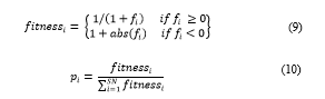
Figure 3: Bitcoin close price

Figure 3 shows the historical movement of bitcoin prices, while figure 4 shows the historical movement of bitcoin trading volume. Highest bitcoin price and volume of bitcoin trading throughout history occurred in December 2017. Bitcoin prices and bitcoin trading volume were used as features in this research.

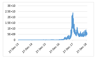Figure 4: Bitcoin traded volume

4.2.  Data Normalization

In this step the dataset value was converted into data with a scale from 0 to 1 using MinMaxScaler in a Scikit Learn library. The dataset after normalization can be seen in table 3. The dataset was divided into 3 sections consisted of 80% training dataset, 10% validation dataset and 10% test dataset. Illustration of bitcoin price dataset after normalized can be seen in table 3.

Table 3: Illustration of normalized bitcoin price dataset

Date	Open	High	Low	Close	Volume	Market Cap
27-Dec-13	0.03038	0.02846	0.02883	0.02883	0.00185	0.02009
28-Dec-13	0.02907	0.02693	0.02839	0.02846	0.00124	0.01983
29-Dec-13	0.02856	0.02701	0.02888	0.02935	0.00068	0.02048
30-Dec-13	0.02925	0.02791	0.03025	0.02992	0.00075	0.02090
31-Dec-13	0.03023	0.02761	0.03014	0.02981	0.00076	0.02082

4.3.  Feature

Features that were used in this research consisted of the closing price of bitcoin and the volume of bitcoin traded as seen in table 4.

Table 4: Features

Feature	Description
P	Bitcoin close price
V	Bitcoin traded volume
Y	Predicted Bitcoin price

4.4.  Hyperparameter

In this step, hyperparameters selection were determined, along with variations in values. This optimized hyperparameters had a significant effect on the performance of the LSTM model. This research optimized 7 hyperparameters with varying values. Breuel [27] and Greff et al. [28] compared the LSTM performance using various hyperparameters, and concluded that one of the most important hyperparameter was learning rate, because it had direct impact to model performance. Selected hyperparameters and the range values in this research can be seen in table 5.

Table 5: List of optimized hyperparameter

No	Hyperparameter	Range Value	Interval
1	Sliding Window Size	40 – 70	5
2	Number of LSTM Units (neurons)	30 – 100	5
3	Dropout	0.3 – 0.5	0.01
4	Learning Rate	0.0001 – 0.01	0.0001
5	Regularizer	L1, L2, L1L2	–
6	Regularizer Rate	0.005 – 0.02	0.001
7	Optimizer	rmsprop, adam, nadam	–

4.5.  Environment and Parameter Setting

These experiments were conducted on Google Colab using GPU accelerator. The models were created using TensorFlow. TensorFlow is an open source deep learning framework that is widely used for research and production. In this research were performed 30 experiments, where each experiment consistsed of approximately 210 models and each model used 512 batch size and 1.000 epochs.

ABC algorithm in this experiment used the parameter setting as in the table 6.

Table 6: ABC parameter setting

Parameter	Setting
Dimension	7
Solution Number	10
Population Size	20
Limit	7
Maximum Cycle Number	10

4.6.  Evaluation

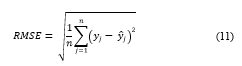
For evaluating the performance of all models with different hyperparameter combination that was performed in the ABC optimization, Root Mean Squared Error (RMSE) was used. RMSE is calculated using Eq. (11). RMSE is often used to evaluate the predictions of forecasting activities. The smaller the RMSE value, the more accurate the predictions.

4.7.  Experiment result obtained using ABC-LSTM

Figure 5 shows the convergence process of ABC-LSTM in obtaining a combination of hyperparameter that produced a prediction with the smallest RMSE value. From 30 experiments, where each experiment consisted of approximately 210 models, result 30 best models, the first ABC-LSTM best model was selected that produced the smallest RMSE value 183.342117450547. The first ABC-LSTM best model had hyperparameter as follows:

• Sliding window size = 60
• Number of LSTM neurons = 65
• Dropout = 0.31
• Learning Rate = 0.0091
• Regularizer = L2
• Regularizer Rate = 0.014
• Optimizer = RMSprop

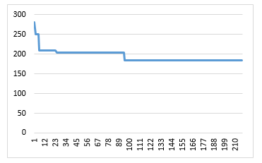Figure 5: Convergence of the selected ABC-LSTM best model

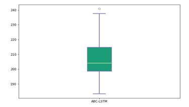Figure 6: Boxplot of 30 ABC-LSTM best model performance

Figure 6 shows the boxplot of 30 ABC-LSTM best model from 30 experiments while table 7 shows the descriptive statistics of the RMSE of ABC-LSTM best model ​​from each experiment. Smallest RMSE value obtained is 183.3421175 and biggest RMSE value obtained is 240.8371386.

4.8.  Comparison with LSTM without optimization

After obtaining the best combination of hyperparameter, comparisons conducted to model that use LSTM without optimization or using standard hyperparameter. For model without optimization there were 7 experiments with sliding windows of 5, 10, 20, 40, 60, 80 and 100, each with 60 runs. For the first ABC-LSTM best model also with 60 runs.

Table 7: 30 ABC-LSTM best  model performance

Measure	ABC-LSTM
Mean	206.8833373
Standard Deviation	13.31792151
Best	183.3421175
Worst	240.8371386

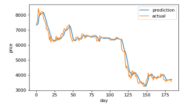Figure 7: LSTM (5) prediction and actual comparison

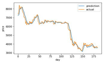Figure 8: LSTM (10) prediction and actual comparison

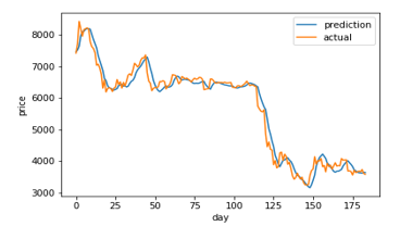Figure 9: LSTM (20) prediction and actual comparison

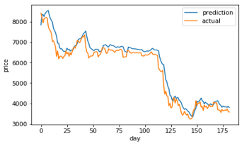Figure 10: LSTM (40) prediction and actual comparison

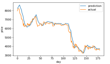Figure 11: LSTM (60) prediction and actual comparison

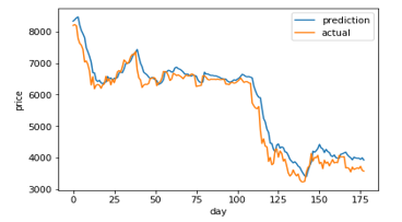Figure 12: LSTM (80) prediction and actual comparison

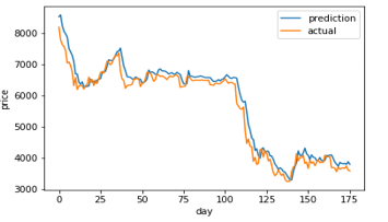Figure 13: LSTM (100) prediction and actual comparison

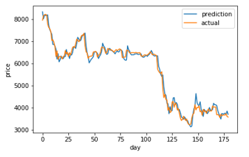Figure 14: ABC-LSTM prediction and actual comparison

Figure 7-14 shows a comparison graph between the actual price and the prediction price of bitcoin using model that use LSTM without optimization, and the first best ABC-LSTM model. ABC-LSTM model shows most similarity between prediction and actual price.

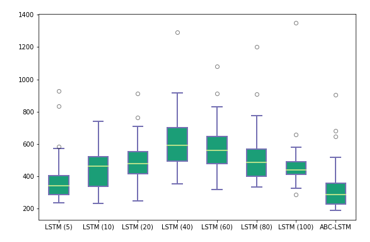Figure 15: Boxplot of comparison with benchmark models

Table 8: Performance comparison

Model	Mean	Deviation Std	Best	Worst
LSTM (5)	368.62	125.94	236.17	929.33
LSTM (10)	437.88	114.34	233.66	740.96
LSTM (20)	488.13	124.33	246.52	912.74
LSTM (40)	611.44	162.23	351.73	1292.90
LSTM (60)	570.79	143.95	316.88	1080.47
LSTM (80)	503.91	145.46	332.63	1201.08
LSTM (100)	461.99	133.54	287.08	1347.78
ABC-LSTM	315.96	131.02	189.61	903.01

Figure 15 shows boxplot of comparison of model that use LSTM without optimization and the first ABC-LSTM best model. Prediction using the first ABC-LSTM best model produced the smallest RMSE value of 189.61. It also produced the lowest average RMSE value of 315.96. Performance of other models can be seen in table 8.

5. Conclusion

There were 2 features used in this study, bitcoin prices and bitcoin traded volume and 7 hyperparameters consisted of sliding window size, number of LSTM units, dropout, learning rate, regularizer, regularizer rate, and optimizer. From 30 ABC-LSTM experiments, the selected ABC-LSTM best model resulted RMSE of 183.34. The best ABC-LSTM model resulted best RMSE of 189.61 compared to models that use LSTM without optimization resulted best RMSE of 236.17. This result showed that ABC-LSTM model outperformed models that use LSTM without optimization.

Besides ABC, another metaheuristic that is very popular used for optimization is genetic algorithm (GA). GA is one of the evolutionary algorithms where best solutions will be used as parents. Those best solutions will be bred to produce a new solution that is better than the parent solutions. In the next research, a comparison between optimizing hyperparameter on models that use LSTM using ABC and GA will be performed.

1.  S. O. Adebiyi, A. A., Ayo, C. K., Adebiyi, M. O., & Otokiti, “Stock Price Prediction using Neural Network with Hybridized Market Indicators,” J. Emerg. Trends Comput. Inf. Sci., vol. 3, no. 1, pp. 1–9, 2012.
2.  E. Guresen, G. Kayakutlu, and T. U. Daim, “Using artificial neural network models in stock market index prediction,” Expert Syst. Appl., vol. 38, no. 8, pp. 10389–10397, 2011.
3.  H. Jang and J. Lee, “An Empirical Study on Modeling and Prediction of Bitcoin Prices With Bayesian Neural Networks Based on Blockchain Information,” IEEE Access, vol. 6, no. 99, pp. 5427–5437, 2018.
4.  S. McNally, J. Roche, and S. Caton, “Predicting the Price of Bitcoin Using Machine Learning,” Proc. – 26th Euromicro Int. Conf. Parallel, Distrib. Network-Based Process. PDP 2018, pp. 339–343, 2018.
5.  L. Alessandretti, A. ElBahrawy, L. M. Aiello, and A. Baronchelli, “Anticipating cryptocurrency prices using machine learning,” Complexity, vol. 2018, pp. 1–16, 2018.
6. D. Chhachhiya, A. Sharma, and M. Gupta, “Designing optimal architecture of recurrent neural network (LSTM) with particle swarm optimization technique specifically for educational dataset,” Int. J. Inf. Technol., vol. 11, no. 1, pp. 159–163, 2019.
7.  H. Chung and K. Shin, “Genetic Algorithm-Optimized Long Short-Term Memory Network for Stock Market Prediction,” Sustainability, vol. 10, no. 10, p. 3765, 2018.
8.  A. ElSaid, F. El Jamiy, J. Higgins, B. Wild, and T. Desell, “Using ant colony optimization to optimize long short-term memory recurrent neural networks,” Proc. Genet. Evol. Comput. Conf. – GECCO ’18, pp. 13–20, 2018.
9.  J. Huisu, J. Lee, and W. Lee, “Predicting Bitcoin Prices by Using Rolling Window LSTM model,” ACM, 2018.
10.  D. Karaboga and B. Basturk, “A powerful and efficient algorithm for numerical function optimization: Artificial bee colony (ABC) algorithm,” J. Glob. Optim., vol. 39, no. 3, pp. 459–471, 2007.
11.  B. Akay and D. Karaboga, “A modified Artificial Bee Colony algorithm for real-parameter optimization,” Inf. Sci. (Ny)., vol. 192, pp. 120–142, 2012.
12.  D. Karaboga, B. Akay, and C. Ozturk, “Artificial Bee Colony (ABC) Optimization Algorithm for Training Feed-Forward Neural Networks,” Modeling Decisions for Artificial Intelligence, pp. 318–329, 2007.
13.  D. Karaboga and C. Ozturk, “A novel clustering approach: Artificial Bee Colony (ABC) algorithm,” Appl. Soft Comput. J., vol. 11, no. 1, pp. 652–657, 2011.
14. M. Mernik, S. H. Liu, D. Karaboga, and M. Črepinšek, “On clarifying misconceptions when comparing variants of the Artificial Bee Colony Algorithm by offering a new implementation,” Inf. Sci. (Ny)., vol. 291, no. C, pp. 115–127, 2015.
15.  A. Saxena, T. R. Sukumar, T. Nadu, and T. Nadu, “Predicting bitcoin price using lstm And Compare its predictability with arima model,” Int. Journa Pure Appl. Math., vol. 119, no. 17, pp. 2591–2600, 2018.
16.  X. Zhan, Y. Li, R. Li, X. Gu, O. Habimana, and H. Wang, “Stock Price Prediction Using Time Convolution Long Short-Term Memory Network,” KSEM, vol. 11061, pp. 461–468, 2018.
17.  S. Borovkova and I. Tsiamas, “An Ensemble of LSTM Neural Networks for High-Frequency Stock Market Classification,” Journal of Forecasting, pp. 1–27, 2018.
18.  T. Fischer and C. Krauss, “Deep learning with long short-term memory networks for financial market predictions,” Eur. J. Oper. Res., vol. 270, no. 2, pp. 654–669, 2018.
19.  T. Gao and Y. Chai, “Improving Stock Closing Price Prediction Using Recurrent Neural Network and Technical Indicators,” Neural Comput., vol. 30, no. 10, pp. 2833–2854, 2018.
20.  D. M. Q. Nelson, A. C. M. Pereira, and R. A. De Oliveira, “Stock market’s price movement prediction with LSTM neural networks,” in Proceedings of the International Joint Conference on Neural Networks, 2017, vol. 2017, pp. 1419–1426, 2017.
21.  N. I. Indera, I. M. Yassin, A. Zabidi, and Z. I. Rizman, “Non-linear Autoregressive with Exogeneous input (narx) bitcoin price prediction model using PSO-optimized parameters and moving average technical indicators,” J. Fundam. Appl. Sci., vol. 9, no. 3S, p. 791, 2018.
22. S. Yunbeom and Changha Hwang, “Predicting Bitcoin Market Trend with Deep Learning Models,” Quant. Bio-Science, vol. 37, no. 1, pp. 65–71, 2018.
23.  M. Sheikhan and N. Mohammadi, “Time series prediction using PSO-optimized neural network and hybrid feature selection algorithm for IEEE load data,” Neural Comput. Appl., vol. 23, no. 3–4, pp. 1185–1194, 2013.
24.  S. Sun, Y. Wei, and S. Wang, “AdaBoost-LSTM Ensemble Learning for Financial Time Series Forecasting,” in International Conference on Computational Science, pp. 590–597, 2018.
25.  N. K. Manaswi, Deep Learning with Applications Using Python. Berkeley, CA: Apress, 2018.
26.  Z. Zhao, W. Chen, X. Wu, P. C. Y. Chen, and J. Liu, “LSTM network: a deep learning approach for short-term traffic forecast,” IET Intell. Transp. Syst., vol. 11, no. 2, pp. 68–75, 2017.
27.  T. M. Breuel, “Benchmarking of LSTM Networks,” J. Cryst. Growth, vol. 285, no. 4, pp. 486–490, 2015.
28.  K. Greff, R. K. Srivastava, J. Koutník, B. R. Steunebrink, and J. Schmidhuber, “LSTM: A Search Space Odyssey,” IEEE transactions on neural networks and learning systems, pp. 1–11, 2016.

(Click Here)

(Click Here)