1. Introduction

Model predictive control (MPC) is a technique that can be used to calculate feedback control for both linear and nonlinear systems using online optimisation techniques. Due to its great flexibility, MPC is likely to be the method with the most practical applications among modern control algorithms. MPC is suitable for limited, multivariable systems and for control problems where regulation of the control function is very difficult or even impossible. One of the great advantages of MPC is its ability to handle the limitations of the system, which makes these methods very interesting to industry.

Linear control theory generally deals with systems that are defined in continuous time and that can be described by ordinary differential equations in which the process model is the cornerstone of MPC. The model should fully capture the process dynamics and also be set up so that the predictions can be calculated.

The application of MPC to mechatronic systems for servo design attracts the attention of many scientists because of the continuous development of microprocessor technology. Mechatronic systems such as electrical motor control [1], two-stage actuation system control and machine tool chattering control [2] have shown promising results. Various advanced techniques are being rapidly developed that integrate MPC to improve performance [3]. However, the sampling frequencies previously used in the research literature may be too low for general mechatronic systems. Moreover, simulations show that the existence of modelling errors leads to obvious steady-state errors. Both of these points, especially during real-time implementation, may influence the performance of mechatronic systems. For example, the calculation of the solution of MPC tech-    niques in an off-line explicit way has been demonstrated [4, 5], and MPC has been also applied to piezoelectric actuators [6]. Finding the conditions for stability is one of the interesting issues in optimisation.

The goal of this paper is to find the lower bounds of a matrix characterising the cost function that gives stability in an optimal solution. The results obtained by means of a proportional integral (PI) controller by Mercorelli et al. [7] and Mercorelli [8, 9] are extended in this contribution. This work considers a water distillation system in which water is separated from mud and impurities using a standard solution based on a heating system combined with a pressure control structure. The experimental setup represents a good example in terms of sustainability. Nevertheless, the algorithm proposed can be applied to any other linear system and represents an advancement in terms of the choice of weighting parameters for the cost function.

The paper is organized as follows. Section 2 is dedicated to model a water recovery system. Section 3 presents backgrounds of MPC. In Section 4 and 5, the structure of LGMPC is analysed without and with input saturation respectively. In Section 6, the proposed control technique is applied to a simulated example in the context of a Water Recovery Process. Conclusion closes the paper.

2. Mathematical model of the system

Figure 1 shows a schematic of the system being considered. The system comprises three elements: a boiler, a compressor and an evaporator. The waste water is located in the middle of the boiler.

The main nomenclature min(t): input mass flow (kg/sec) mo(t): output mass flow (kg/sec) m(t): mass (Kg) dm(t) : mass flow (kg/sec) dt p(t): pressure inside the evaporator (Pa) T: temperature (K) V: volume (l) pi: initial pressure (Pa) pd: desired pressure (Pa) Rg: vapour constant Aw: anti-windup signal Kb: weight factor for the anti-windup action VL: a Lyapunov function Ak: discrete system matrix Bk: discrete input matrix Hk: output matrix Gp: model predictive control state matrix F1p: model predictive control ”delta” input matrix F2p: model predictive control input matrix

A vapour chamber hosts water vapour produced by heating the waste water in the upper part. In the first phase, the resistor system heats the waste water. After that, vapour appears in the chamber. The heating process is then turned off and the compressor is turned on. The pressure in the vapour chamber must be reduced using the compressor with the help of a mass flow. This mass flow (m₀(t)) represents cleaned and distilled water in the output of the evaporator. To be more precise, the vapour is condensed and transfers heat to the waste water in the evaporator. The low pressure in the vapour chamber allows new waste water to penetrate into the boiler. In this case, the compressor plays the role of a controller, and the mass flow m₀(t), with the constraint that m₀(t) > 0, represents its output. The compressor includes an asynchronous motor being regulated by means of an inverter, which is driven by a pulse-width modulated (PWM) signal that converts the output of the LMPC controller into a frequency. The error signal occurs in the input to the LMPC. The section concerning the simulation demonstrates the details of the control scheme. The dynamics of the asynchronous motor with the inverter and the other converters are not considered in this analysis, but they are faster than the dynamics of the controlled process.

In the first phase, the pressure in the container is approximately 1.013 bar. The pressure increases during heating as the water starts to evaporate. At a lower pressure, the water boils and evaporates faster. New water is added under control. The ”internal heat exchanger” helps to condense the vapour, which now contains no impurities. The controller design must take the dynamic model of the system into account. As explained above, the following equations can be taken into account, considering that the process of regulation begins when the steam is in the boiler. The idealised model can be presented as follows:

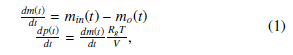with m_in(t) being a stepwise positive constant function.

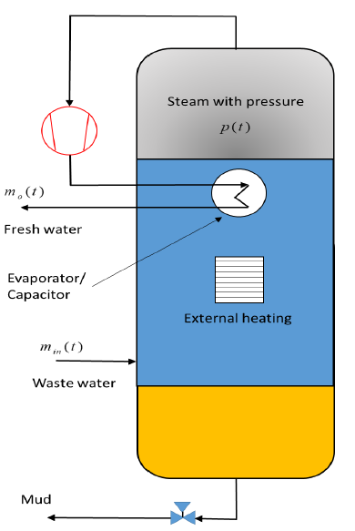Figure 1: Boiler system

Considering the forward Euler discretisation with sampling time T_s, this expression is obtained:

3. Model predictive control

The process model is the cornerstone of MPC. The model should fully capture the process dynamics and also be set up so that the predictions can be calculated. At the same time, it should be intuitive and allow a theoretical analysis. The process model is necessary to calculate the predicted output quantities y(t + k|t), also referred to as outputs, in a future instance, where y(t + k|t) designates the output at time t + k from time t. The various strategies of MPC can use numerous models to show the relationship between the output quantities and the measurable input quantities (inputs). A disturbance model can also be considered to describe behaviour not reflected by the process model, as well as non-measurable input magnitudes, measurement noise and model error. However, we will not consider these models at this point. Virtually any form of modelling in an MPC formulation can be used, but the following are the most common.

3.1    Problem definition and general idea of MPC

The problem of the model-predictive approach is a generalised form of stabilisation: the so-called tracking problem. The goal here is that the output quantities y(t + k) follow a given reference trajectory w(t + k), i.e. the deviation of the output quantities y(t + k) from a known reference trajectory w(t + k) should be minimised within a certain time window (horizon N) in order to keep the process as close as possible to this trajectory. This can be achieved by influencing the future output variables by a control sequence u(t + k) to be calculated within a finite horizon N. For this purpose, a goal function J is set up, which is normally quadratic in form. The reference trajectory w is assumed to be known. The calculated output quantities y(t + k), on the other hand, depend on the chosen model description and the future control signals u(t + k) or the vector of the future control function changes ∆u(t) = u(t) − u(t − 1). The basic idea of MPC can be explained in the following way. The future control quantities y(t + k) at time t are to be predicted over a finite horizon N using the process model. These calculated output quantities depend on known values of the instance t and the future control signals u(t + k), which are to be calculated and output to the system. The future control sequence is calculated by optimising

a certain criterion, in most cases by minimising a target function J. Starting from the current time t, this objective function is now set up over the control horizon N and, with suitable optimisation methods, dependent on the zuk control values u(t + k) and control value changes ∆u are minimised.

3.2    The considered case

Just two samples of the model approach are considered:

where

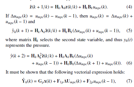
where y_d(k + j), j = 1,2,…, N is the pressure reference profile, N is the prediction horizon, and Q_p and R_p are non-negative definite matrices. Index (17) can be written as

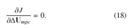
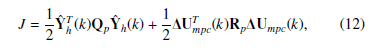where Yˆ ^T_h (k) represents the error between the desired output and the predicted output. The solution minimising performance index (12) may then be obtained by solving

An off-line computation of the solution may be obtained in an explicit form as follows:

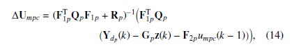where Y_dp (k) is the desired output column vector. For further details see Sunan et al. [10].

4. A stability sufficient constructive condition in GMPC

Theorem 1 Let us consider the discrete SISO linear system:

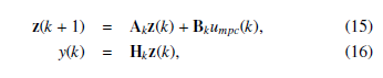obtained by a discretisation of a linear continuous system by means of a sampling time equal to T_s. u_mpc(k) is the first element of the vector of the optimal solution [10] for the GMPC considering the cost function:

where y_d(k + j), j = 1,2,…, N is the position reference trajectory, N is the prediction horizon and Q_p and R_p are non-negative definite matrices. The solution minimising the performance index (17) may be obtained by solving

From Sunan et al. [10], it can be seen that the optimal solution is: umpc(k) = (FT1pQpF1p + Rp)−1FT1pQp

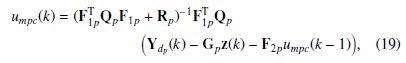where Y_dp (k) and Y_p(k) are the desired output column vector and the measured or observed output vector. Matrices Q_p and R_p are diagonal and positively defined. Under the technical hypotheses that Q_p = I and H^T_k H = I, and the assumption

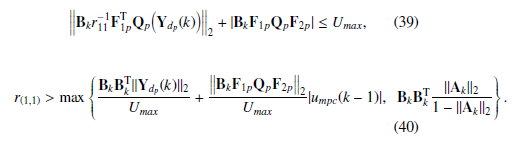
1. i) r_(1,1) >> T_s², where r_(1,1) represents the first diagonal element of matrix R_p, then ∀ r₍₁,₁₎ such that:

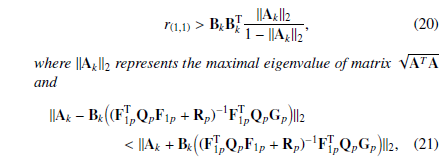Proof Theorem 1 For the sake of brevity, just one prediction step is considered, then:

considering that scalar r_(1,1) > 0 and scalar B_kB^T_k > 0:

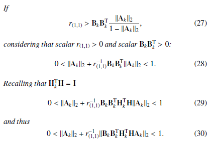With matrix F_1p defined as in (22) and G_1p defined as in (24), it is known that matrix B_k is proportional to T_s, then considering that R_p = r_(1,1), choosing a suitable r_(1,1) >> T_s and considering that Q_p = I (technical hypothesis), this condition is derived:

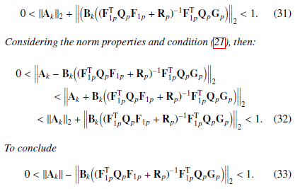The constraint in (27) states a plausible condition on the controller. If mass m → ∞, then, because of the discretisation and according to the Landau notation,     A   → 0 with For a very slow system, according to (27), r_(1,1) → 0, parameter r_(1,1) is present in the denominator function of the optimal solution in (19) and small values of r_(1,1) are devoted to speeding up the system. If mass m → 0, then, because of the discretisation, O(B_kB^T_k ) = O(_m¹₂ ). For a very fast system, r_(1,1) → ∞, parameter r_(1,1) is devoted to slowing down the system. We can therefore conclude that a highly inertial system needs relatively small values of r_(1,1) to be optimised and stabilised. If the inertia is small, then the system needs larger values of r_(1,1) to be optimised and stabilised. In fact, very fast systems can have very high abrupt changes in the input signals and in the cost function, and the input factor needs to be reduced to find an optimality.

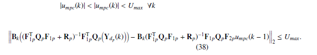
5. The case of input saturation

It is possible to observe that for large values of U_max, the condition on the input barrier in the cost function (17) with weight r_(1,1) is not so restrictive, so larger inputs are allowed. For small values of U_max, the input barrier limits the values of the input and no large input values are allowed.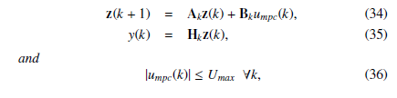

6. Simulation results

It must be clarified that function m_in(t) is a stepwise constant function with m_in(t) = 0.086 (kg/sec) or m_in(t) = 0 and in the simulated case m_in(t) = 0.086 (kg/sec) is considered. Two cases should be differentiated: weak anti-saturating action:

Umax

Figure 2 shows the controlled pressure, which represents the result. If the anti-windup action is relatively weak, more time is necessary to re-establish the control loop. As already explained, during the windup effect, the feedback control is broken. The long period where the pressure is at negative values can be explained by the absence of feedback control action. From Fig. 3, representing the mass flow ^dm_dt^(t) = m_in(t) − m₀(t) (kg/sec), it can be seen that this function is a consequence of the relation:

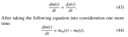After taking the following equation into consideration one more time: dm(t) = m_in(t) − m₀(t), (44) dt for activating the process, a strong initial action through the mass flow m₀(t) is necessary. These two figures show that in case of a strong anti-saturating action in Fig. 5, the controlled system emerges from the saturation state very quickly with faster dynamics thanks to the stronger anti-windup action. After saturation occurs, the control loop becomes open and there is no presence of feedback control.

Figure 2: Desired and obtained pressure with weak anti-saturating action Time (sec)

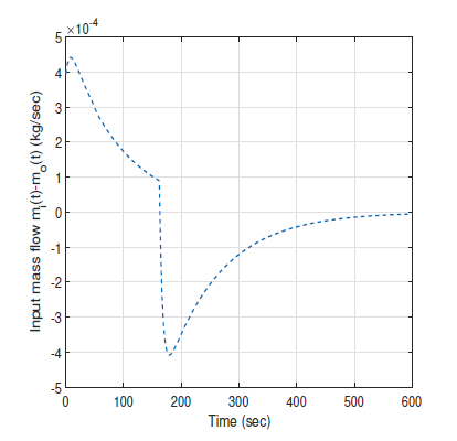Figure 3: Mass flow ^m_dt^(t) = m_in(t) − m₀(t) (kg/sec) with weak anti-saturating action Time (sec)

Figure 4: Desired and obtained pressure with strong anti-saturating action Time (sec)

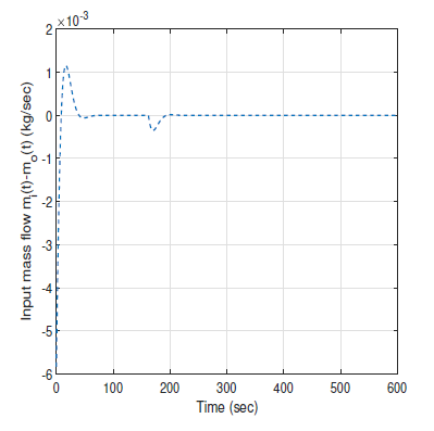Figure 5: Mass flow ^dm_dt^(t) = m_in(t) −m₀(t) (kg/sec) with strong anti-saturating action

7. Conclusion

Conservative conditions for stability are a crucial problem in optimisation using LMPC. This contribution is devoted to a sufficient and constructive condition for the stability of an LGMPC, which calculates a lower bound for the elements of matrix R. The obtained results are physically interpreted. An illustrative example is provided in which a water recovery process is taken into consideration to test the proposed results through computer simulations.

Conflict of Interest     The authors declare no conflict of interest.

1.  Bolognani, S.; Peretti, L.; Zigliotto, M. Design and implementation of model predictive control for electrical motor drives. IEEE Transactions on Industrial Electronics 2009, 56, pp. 1925–1936.
2.  Neelakantan, V.; Washington, G.; Bucknor, N. Model Predictive Control of a Two Stage Actuation System using Piezoelectric Actuators for Controllable Industrial and Automotive Brakes and Clutches. J. Intell. Mater. Syst. and Struct. 2008, 19, pp. 845–857.
3.  Hu, Z.; Farson, D. Design of a waveform tracking system for a piezoelectric actuator. Proc. Inst. Mech. Eng., J. Syst. Control Eng., 2008, Vol. 222, pp. 11–21.
4.  Bemporad, A.; Morari, M.; Dua, V.; Pistikopoulos, E.N. The explicit linear quadratic regulator for constrained systems. Automatica 2002, 38, pp. 3–20.
5.  Pedret, C.; Poncet, A.; Stadler, K.; Toller, A.; Glattfelder, A.; Bemporad, A.; Morari, M. Model-varying predictive control of a nonlinear system. Inter-nal report in Computer Science Dept. ETSE de la Universitat Auto`noma de Barcelona 2000.
6. Liu, Y.C.; Lin, C.Y. Model Predictive Control with Integral Control and Constraint Handling for Mechatronic Systems. Proc. of the 2010 International Conference on Modelling, Identification and Control; , 2010; pp. 424–429.
7. Mercorelli, P.; Goes, J.; Halbe, R. A Lyapunov based PI controller with an anti-windup scheme for a purification process of potable water. Proc. of the 2014 International Conference on Control, Decision and Information Technologies (CoDIT), 2014, pp. 578–583.
8. Mercorelli, P. An Optimal and Stabilising PI Controller with an Anti-windup Scheme for a Purification Process of Potable Water. Proc. of the 16th IFAC Workshop on Control Applications of Optimization CAO’2015, 2015, pp. 259–264.
9.  Mercorelli, P. A sufficient asymptotic stability condition in generalised model predictive control to avoid input saturation. Lecture Notes in Electrical Engi- neering 2019, 489, pp. 251–257.
10.  Sunan, H.; Kiong, T.; Heng, L. Applied Predictive Control; Springer-Verlag London: Printed in Great Britain, 2002.

(Click Here)

(Click Here)