1. Introduction

Load forecasting is a topic of electrical systems which  has been studied for a long time. There are two main approaches in this area: Traditional statistical modeling of the relationship between load and factors affecting load (such as time series, regression analysis, etc) and artificial intelligence, machine learning methods. Statistical methods assume load data according to a sample and try to forecast the value of future loads using different time series analysis techniques. Intelligent systems are derived from mathematical expressions of human behavior / experience. Especially since the early 1990s, neural networks have been considered one of the most commonly used techniques in the field of electrical load forecasting, because it assumes that there is a nonlinear function related to historical values and some external variables with future values may affect the output [1]. The approximate ability of neural networks has made their applications popular.

In recent years, an intelligent calculation method involving Support Vector Machines has been widely used in the field of load forecasting. In 2001, Bo-Juen Chen, Ming-Wei Chang, and Chih-Jen Lin used the Support Vector Regression technique to solve the electrical load prediction problem (forecasting a maximum daily load of the next 31 days). This was a competition organized by EUNITE (European Network on Intelligent Technologies for Smart Adaptive Systems). Information was provided includes: demand data of the past two years, daily temperature of the past four years and local holiday events. Data was divided into 2 parts: a part used for training (about 80 – 90%) and the rest used for algorithm testing (about 20-10%). The set of training inputs included: data of the previous day, the previous hour, the previous week, the average of the previous week. Their approach in fact won the competition [2].

Since then, there have been several studies exploring the different techniques used for optimizing SVR to perform load forecasting [3-10]. The main reason for using SVM in load forecasting is that it can easily model the load curve, the relationship between the load and the dynamics of changing load demand (such as temperature, economic and demographics).

However, there are some problems encountered when the above algorithms apply to reality:

• Climate conditions always play an important role in load forecasting. They show the relationship between climate and load demand, when we do the load forecasting for the post-test period, it is very difficult to forecast the values of weather and climate used as the input of the algorithm and these values are often not available.
• Electrical load samples include hidden elements, which tend to be similar to the previous load model. However, it will lead to a false forecast of the following days if the date pattern is different from the previous day or there is an event that impacts. Therefore, the use of the dataset (training inputs included: data of the previous day, the previous hour, the previous week, the average of the previous week) has many risks if the load models are not identical.
• If the forecast time frame is greater than the past data frame (more than 07 days due to the algorithm data is the previous week’s values), there will be a lack of input to run the algorithm.
• In addition, for Asian countries (such as Vietnam) that use lunar calendar, one of the most difficult and unpredictable issues is the Lunar New Year (usually in late January or early February), or the lunar calendar (Hung King’s Anniversary), etc. There is a deviation between the solar calendar and the lunar calendar (the load models are not identical). Therefore, it often leads the forecast results of algorithm for this period with large errors.

For this reason, the paper proposes a solution to build a Standardized Load Profile (SLP) based on the historical load dataset as a training dataset. This input dataset is combined with the Support Vector Regression algorithm (SVR) to improve the accuracy of short-term forecast results, solve the problem of deviation between the solar and the lunar calendar, as well as overcome the input data frame.

Figure 1: The load profiles of February over the years

SLP will be built for all 365 days and 8,670 cycles in a year. SLP will be an important dataset during training, testing and forecasting process. SLP will be built for all 365 days and 8,670 cycles in 1 year. SLP will be an important set of data during training, testing and forecasting. SLP will standardize load models: by hours, by days, by seasons, and by special day types (including lunar dates). Therefore, SLP will contribute to solve the above-mentioned difficulties and improve the quality of electrical load forecasting.

2. Methodology

Observing the load profiles of February of Ho Chi Minh City over the years (Figure 1), a huge fluctuation in chart shape over the years can be seen. This results in the use of historical data for forecasting this period of time is extremely complicated.

In fact, the algorithms used to forecast in Vietnam have to go through an intermediary which converts these months into regular months (without holidays, Lunar New Year). After being calculated, the forecast result will be reversed or the result will be accepted with a large error. Commercial software provided by foreign countries all have this problem.

2.1.  Standardized Load Profiles (SLP)

The Standardized Load Profile is an electrical load profile according to the relative values, converted from the total power consumption during the electrical load research cycle. The standardized load profle of day / month / year of each electrical load sample is constructed by dividing the load profile of a sample (from the measured data collected by day / month / year) by the power consumption of day / month / year of the sample.

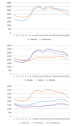Figure 2: Typical load profiles of some days of a year

Considering the load profiles of the days in a week and some special holidays of the year in Ho Chi Minh City area (Figure 2),the difference between weekdays (from Tuesday to Friday) can be ignored and they have the same load chart. For the load profiles on Monday, they are different from the normal days at 0:00 to 9:00, due to the forwarding demand from Sunday.

For load profiles on Saturday, there is  an insignificant change compared to normal days, mainly the load demand decreases in the evening due to the start of the weekends. Particularly for load profiles on Sunday, it is completely different from normal days (the demand for electricity is low).

When observing the load chart of the New Year and Lunar New Year, a noticeable difference can be seen where the graphs are almost flat and the load demand is quite low because these are holidays.Particularly on Lunar New Year, the load demand is the lowest since this is the longest holiday of the year (maybe from 6 to 9 days).

Standardized Load Profiles (SLP) are built by taking the value of the collected capacity in a 60-minute period divided by its maximum capacity. We need to build SLP for 365 days per year. Some typical SLP:

Figure 3: SLP of some days in a year

Based on the SLP of each cycle of the past data set, we can build the SLP data set for future forecast periods. This should be accurate to each cycle, each type of day (holidays, weekdays, working days, holidays, etc.), each week and month.Therefore, the standardized load profiles (SLP) is a special feature and is also an important input parameter of the SVR (NN) machine learning algorithms training process to rebuild the load curves, from which we can estimate the amount of lost or not recorded data  during the measurement process.

2.2.  Support vector regression (SVR)

The SVM was proposed by Vapnik in [7] to solve the data classification problem. Two years later, the proposed version of SVM was successfully applied to non-linear regression problems. This method is called support vector regression (SVR) and it is the most common form of SVMs.

The goal of SVR is to create a model that predicts unknown outputs based on known inputs. During training, the model is formed based on the known training data set (x₁, y₁), (x₂, y₂), …, (x_n, y_n), where x_i is input vectors and y_i is output vectors. During the test period, the model was trained on the basis of new inputs x₁, x₂, …, x_n to make predictions about unspecified outputs y₁, y₂, …, y_n.

Consider a known training set {x_k, y_k}, k = 1, …, N with input vectors x_k ∈ Rn and scalar output vectors y_k ∈ R. The following regression model can be developed by using the nonlinear mapping function φ (.): R_n → R_nh to map the input space into a multidimensional characteristic space and build linear regression in it, as shown in (1):

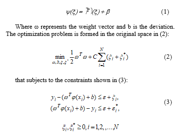where xi is mapped in a multidimensional vector space with the mapping φ, ξ_i is the upper limit of the training error and  is lower. C is the constant that determines the error cost, that is, the tradeoff between the complexity of the model and the accepted larger degree of error. The parameter ε includes the width of the non-sensitive area, which is used to match the training data [7-10]. The parameters C and ε are not known in advance and must be determined by some mathematical algorithm applied on the training set (eg Grid – Search and Cross – Validation). The goal of the SVR is to place many input vectors x i inside the pipe , shown in Figure 4. If the xi is not in the tube, the errors ξi, will occur.

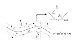Figure 4: ε tube of nonlinear SVR

To solve the optimization problem identified by (2) and (3), it is necessary to develop a dual problem using Lagrange function, the weight vector ω and the deviation b. The SVM results for the regression model in the double form are shown in (4), where α_i and  are the Lagrange multipliers, K (x_i, x) represents the Kernel function, defined as a midpoint và .

The Kernel functions allow the calculation of dot product in a feature space of height using the input data from the original space, without explicit computation φ (x). The Kernel function is often used in non-linear regression problems, which is used in this study, as the radial basis function (RBF) presented in (5):

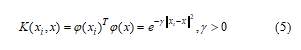where γ represents the Kernel parameter, which should also be determined by mathematical algorithms. More information about SVR can be found in [5] – [6], [11] – [12].

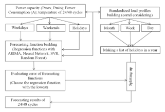Figure 5: Flowchart of forecasting algorithm by SLP – SVR

2.3.  Research models

Processed historical data (power consumption, capacity, temperature recorded at 24 cycles – 60 minutes each) with the Standardized load Profiles (SLP) will be included in modules to build regression functions under SVR (Support Vector Regression), NN (Neural Network) algorithms to build regression functions.

Then we use the above data set to check and evaluate the error of regression functions. After that we choose the regression function with the smallest error which will be used as regression function for the next forecast phase.

The SLP data set in 24 cycles of the expected period (including holidays, etc.) and the forecasted temperature in 24 cycles of the corresponding period will be the input for the regression function that is selected to export forecast results in 24 cycles for a period of 7 – 30 days.

3. Results and Discussion

3.1.  Input data:

The article uses data from January 1, 2015, to November 17, 2018, of EVNHCMC to run test models. After pretreatment, the data set is divided into 2 volumes: training set and test set, in which the test set is the last 30 days of the data set. Or the data set is divided into phases to test the forecast results in different time periods.

Input data for training algorithms include: capacity (Pmax/Pmin) in 60-minute cycles; temperature (max / min) in 60-minute cycles;  standardized load profiles of 24 hours of day; list of holidays and Lunar New Year in the forecast year.

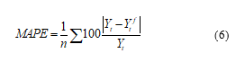
A useful measurement parameter is the mean absolute percentage error (MAPE) which is used to evaluate the error of models.

The algorithms are programmed in Mathlab language and the results are exported to Excel files for data exploitation.

3.2.  SVR Models

Processed historical data (power consumption, capacity, temperature recorded at 24 cycles – 60 minutes each) with the Standardized load Profiles (SLP) will be included in modules to build SVR models, with: normalization coefficient C, width of pipe ε and Kernel function; 4 typical SVR model parameters are proposed:

Table 1: SVR model parameters

Model	C – BoxConstraint	ε – Epsilon	KernelFunction
SVR 1	93.42	32.5	Polynomial
SVR 2	500.32	0.01	Gaussian
SVR 3	1	50.03	Linear
SVR 4	100	0.01	Linear

Define abbreviations and acronyms the first time they are used in the text, even after they have been defined in the abstract. Do not use abbreviations in the title or heads unless they are unavoidable.

3.3.  RFR models

A set of regression trees with each set of different rules to perform non-linear regression. The algorithm builds a total of 20 trees, with a minimum leaf size of 20. The size of leaves is smaller or equal to the size of the tree to control overfitting and bring about high performance [13] – [14]. The algorithm uses the same input data set of models.

RFR model (Random Forest Regression) is a method of constructing regression models from historical data and is also a machine learning method like current advanced models. Therefore it is used as a result to compare with the proposed SVR model.

3.4.  Neural Network Models

We use Feedforward Neural Network models with the input variables and training data set as above. A-hidden-layer network architecture with class size of 10 and Sigmoid activation function is used. At the same time, the usual Neural network with  3-hidden-layer network architecture, in which: the first hidden layer has a size of 10; The second hidden layer has a size of 8 and the third hidden layer has a size of 5.

FNN model (Feedforward Neural Network) is a method of constructing regression models from historical data and is also a machine learning method like current advanced models. Therefore it is used as a result to compare with the proposed SVR model.

4. Results and Analysis

Run the forecast results for February 2018 (the month of the Lunar New Year) to assess the degree of error of the models

4.1.  The model with inputs included: data of the previous day, the previous hour, the previous week and the average of the previous week

Processed historical data (power consumption, capacity, temperature recorded at 24 cycles – 60 minutes each) with the Standardized load Profiles (SLP) will be included in modules to build regression functions under SVR,Neural Network and Random Forest algorithms to build regression functions.

Table 2: Results of checking errors of regression models

Date	Ytr	Yts1	Yts2	Yts3	Yts4	YtNN	Ytfeed	YtRF
23/1/18	9.71	4.05	5.02	6.35	4.19	6.09	4.55	2.91
24/1/18	8.30	3.65	2.61	7.00	4.25	0.65	4.76	4.19
25/1/18	7.17	4.35	3.57	7.42	4.21	4.58	5.84	4.63
26/1/18	7.10	6.20	6.77	7.48	6.39	6.58	5.82	6.44
27/1/18	9.22	1.37	0.44	3.27	1.33	0.56	1.91	1.06
28/1/18	9.68	2.16	3.28	7.12	0.32	25.51	5.89	3.93
29/1/18	9.15	5.30	6.17	6.92	4.91	5.71	5.96	5.67

We choose the regression function with the smallest error whichwill be used as regression function for the next forecast phase.The model Yts4 is selected to be a forecasting model.

• Forecast results for February 2018

Considering the forecast results for February of the model, we see a big difference between reality and forecasting. The reason is that we used the historical data of January 2019 (7-14-30 days before the forecasting date) as the input for the training model.

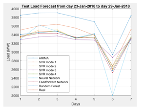Figure 6: Regression models test

Figure 7: Forecast results for the next 30 days

4.2.  SLP – SVR combination model

Processed historical data (power consumption, capacity, temperature recorded at 24 cycles – 60 minutes each) with the Standardized load Profiles (SLP) will be included in modules to build regression functions under SVR, Neural Network and Random Forest algorithms to build regression functions

• Results of testing SVR models

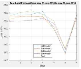Figure 8: SVR models test

Table 3: Results of checking errors of SVR models

Date	Yts1	Yts2	Yts3	Yts4
23/1/18	1.15	0.64	2.22	3.87
24/1/18	1.70	2.12	2.95	6.19
25/1/18	3.03	3.30	3.38	6.68
26/1/18	1.35	1.04	1.76	2.76
27/1/18	6.77	4.56	6.42	1.56
28/1/18	4.18	5.09	1.81	0.76
29/1/18	0.24	0.12	2.69	2.14
MAPE	2.63	2.41	3.03	3.42

• Results of testing machine learning models

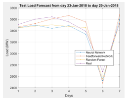Figure 9: Machine learning models test

Table 4: Results of checking errors of machine learning models

Date	YtNN	YtFeed	YtRF
23/1/18	1.25	1.61	1.70
24/1/18	2.14	2.90	3.36
25/1/18	0.99	5.55	3.89
26/1/18	3.16	1.84	2.26
27/1/18	4.81	1.56	1.92
28/1/18	7.51	5.85	4.68
29/1/18	4.41	2.05	0.43
MAPE	3.47	3.05	2.60

• Results of testing regression models:

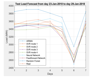Figure 10: Regression models test

Table 5 – Results of checking errors of all models

Date	Ytr	Yts1	Yts2	Yts3	Yts4	YtNN	Ytfeed	YtRF
23/1/18	9.71	1.15	0.64	2.22	3.87	1.25	1.61	1.70
24/1/18	8.30	1.70	2.12	2.95	6.19	2.14	2.90	3.36
25/1/18	7.17	3.03	3.30	3.38	6.68	0.99	5.55	3.89
26/1/18	7.10	1.35	1.04	1.76	2.76	3.16	1.84	2.26
27/1/18	9.22	6.77	4.56	6.42	1.56	4.81	1.56	1.92
28/1/18	9.68	4.18	5.09	1.81	0.76	7.51	5.85	4.68
29/1/18	9.15	0.24	0.12	2.69	2.14	4.41	2.05	0.43
MAPE	8.62	2.63	2.41	3.03	3.42	3.47	3.05	2.60

The results in this Table 5 is the test run results of the regression models being developed. The evaluation of the MAPE results of the models aims to select a standard model for the official forecasting model in the later stage. Considering models Yts2 (2.41%) and YtRF (2.60%), they all have quite low error results. However, when considering the error according to each component, the model Yts2 has more advantages and the error of each component is also lower than YtRF. Therefore, it is appropriate for the author to choose the model Yts2.

We choose the regression function with the smallest error which will be used as regression function for the next forecast phase.The model Yts2 is selected to be a forecasting model.

• Forecast results for February 2018

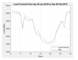Figure 11: Forecast results for the next 30 days

5. Conclusion

Observe the experimental results in the forms of testing datasets (load data sets of the previous day, the previous week, the previous month and the dataset of Standardized Load Profile – SLP), we see the results of the SLP-SVR model are close to the actual value of February 2018, while the results of the old model are in quite large deviation.

Thus, through experimentation, we see that the use of Standardized Load Profile (SLP) as the input dataset for modules of the forecasting regression function is effective and give forecasting results with low errors. It solves the problem of deviation between the solar and the lunar dates, especially in the months of lunar new year, as well as resolving the difference between the solar and lunar cycles.

1.  M H M R ShyamaliDilhani and ChawalitJeenanunt, Daily electric load forecasting: Case of Thailand. 7th International Conference on Information Communication Technology for Embedded Systems 2016 (IC-ICTES 2016). 978-1-5090-2248-9/16/$31.00 ©2016 IEEE.
2.  Juan Huo,Tingting Shi and Jing Chang, Comparison of Random Forest and SVM for Electrical Short-term Load Forecast with Different Data Sources. 978-1-4673-9904-3/16/$31.00 ©2016 IEEE.
3.  Lemuel Clark P. Velasco, Christelle R. Villezas and Jerald Aldin A. Dagaang, Next Day Electric Load Forecasting Using Artificial Neural Networks. 8th IEEE International Conference Humanoid, Nanotechnology, Information Technology Communication and Control, Environment and Management (HNICEM). The Institute of Electrical and Electronics Engineers Inc. (IEEE) – Philippine Section 9-12 December 2015 Water Front Hotel, Cebu, Philippines.
4.  Electricity Load Forecasting for the Australian Market Case Study version 1.3.0.1 by David Willingham. https://www.mathworks.com/matlabcentral.
5.  Nguyen Tuan Dung, Tran Thu Ha, Nguyen Thanh Phuong, Page(s):90 – 95. 10.1109/GTSD.2018.8595514. 2018 4th International Conference on Green Technology and Sustainable Development (GTSD).
6.  E. Ceperic, V. Ceperic, and A. Baric, A strategy for short-term load forecasting by support vector regression machines, IEEE Transactions on Power Systems, vol. 28, pp. 4356–4364, Nov. 2013.
7.  V.Vapnik, 1995, “The nature of statistical learning theory,” Springer, NY.
8.  S.R. Gunn, 1998: Support Vector Machines for Classification and Regression, Technical Report, Image Speech and Intelligent Systems Research Group, University of Southampton.
9.  V. Cherkassky, Y. Ma, 2002: Selection of Meta-parameters for Support Vector Regression, International Conference on Artificial Neural Networks, Madrid, Spain, Aug. pp. 687 – 693.
10. D. Basak, S. Pal, D.C. Patranabis, Oct. 2007: Support Vector Regression, Neural Information Processing – Letters and Reviews, Vol. 11, No. 10, pp. 203 – 224.
11.  A.J. Smola, B. Schölkopf, Aug. 2004: A Tutorial on Support Vector Regression, Statistics and Computing, Vol. 14, No. 3, pp. 199 – 222. 0960-3174 ©2004 Kluwer Academic Publishers.
12.  Understanding Support Vector Machine Regression and Support Vector Machine Regression, http://www.mathworks.com.
13.  Breiman L.: Random Forests. Machine Learning 45 (1), 5-32 (2001). http://dx.doi.org/10.1023/A:1010933404324.
14.  Breiman, L., Friedman, J.H., Olshen, R.A., and Stone, C.J. Classification and Regression Trees, Wadsworth, Belmont, CA, 1984. Since 1993 this book has been published by Chapman & Hall, New York.

(Click Here)

(Click Here)