1. Introduction        

This paper is an extension of the work [1] originally presented in the for new material and new production methods, including tools and 4th International Conference on Computing Science (ICCS),2018. techniques altered for the manufacturing, inspection, reusing and This extended research work incorporates the green inventory conremanufacturing. In [5], the author provided a comprehensive and cept. The harmful effects of the waste and outdated products are immense knowledge for the remanufacturing process from the liter-imposing a threat to the environment. In present scenario, world is ature surveyed. The supplier and retailer are stationed far from each facing pollution as a big hazard to mankind. Every organization is other so it is not possible for the supplier to send all perfect goods. moving towards reducing and reusing the waste/imperfect goods.

In Thus to be assure of the brand and quality, retailer screens the lot this direction this EOQ model aims at a single stage remanufacturing as it is received. In [6], the authors studied the remanufacturing process where the imperfect goods after screening are taken back of the imperfect items to maximize the total profit. The effect of by the supplier and are remanufactured. This is again transported to deterioration is dominant and its consequences cannot be ignored the retailer. Replenishment schedule is derived for the retailer and while framing an EOQ model. Electronic goods, blood, fruits, grain the supplier, considering green product life cycle and the time value products, alcohol are some of the deteriorating products. In [7], the of money. Various countries have adopted several measures for authors were the first to study deterioration in an inventory model.

waste product management, reusing and remanufacturing programs. Several researchers as [8], [9], [10]. [11] studied different patterns International standards as European Union’s proposal for Waste of deterioration in inventory models. In [12], the authors developed Electrical and Electronic equipment (WEEE) introduces the concept an inventory model for the stock dependent demand for deteriorat- of product design, to bring a decrease in the cost of disassembly ing products under two level credit. In [13], the researcher studied a

and remanufacturing [2]. Product, if designed significantly reduces two-echelon supply chain model for deteriorating products under the cost of inspection, disassembly, repair, remanufacturing and trade credit. They analyzed two models, one with demand being recycling. In [3], the author first determine an optimal ordering size stock dependent and the second with de and being selling price with recovery and remanufacturing. He studied the traditional EOQ dependent for the perishable products. In [14], the authors studied model with continuous and deterministic demand and return. In [4], an inventory model for the deteriorating products where the deterioration being time dependent. They studied permissible delay policy in their model. Partially backlogged shortages were als incorporated. In [15], the authors discusses the inventory model for perishable items where deterioration follows exponential distribution under permissible delay.

In conventional EOQ model, assumes that the retailer must pay for the goods as they arrive. But as practice, sometimes the supplier allows permissible delay to the retailer for the settlement of the goods. Numbers of research papers have been published with inventory models under trade credit. The rudest approach of an inventory model under trade credit was done by [16]. [17], developed an EOQ model under two level supply chain with trade credit for deteriorating products and demand being stock dependent. In [18],[19], the authors revisited the inventory models with time and stock dependent demand for imperfect and perishable products allowing trade credit. [20] studies the effect of sales effort on demand in a supply chain inventory model when permissible delay is allowed. He also included quantity discounts in his model with two level supply chain. Trade credit is widely used by the industries in U.S., China and Europe as discussed in [21],[22] and [23]. Suppliers give credit period to the retailer to postpone their payments, thereby increasing their participation and retaining the market. On the other hand, retailer can collect the revenue of the goods during the credit period and is encouraged to increase the order quantity.The concept of trade credit incorporated with the green inventory and weibull deterioration was studied by [24]. In [25], the authors analyses an inventory system with trade credit for imperfect goods and demand being quality dependent. He has considered two different approaches of trade credit in the supply chain model.

The formal EOQ Model establishing various results does not include the inflation for all the inventory related costs, whereas its effect should not be ignored. The first initiation for an inventory model under the time value of money was considered by [26]. In [27], the researchers analyzed an inventory model with the time value of money and weibull deterioration. In [28], the authors proposed a deteriorating EOQ model when demand is poisson and lead time is non zero. In [29], the authors developed a replenishment model for perishable products with return policy under inflation. In [30], the authors determine a reordering policy in an inventory model for deteriorating goods,partial backordering under inflation. In [1], the authors represented supply chain inventory model with inflation for time quadratic demand and deterioration. In [31], the authors developed an inventory model for deteriorating products considering inflation in a green supply chain for remanufacturing and recycling. Also a fuzzified model was developed by [32].

2. Assumptions and Terminology

2.1    Assumptions

The following assumptions are followed:

1. All inventory related cost are subjected to the same constant rate of inflation r.
2. The supplier offers the retailer credit period ρ to settle the account.
3. Finite replenishment and non zero lead time is considered.
4. The available inventory deteriorates with a constant fraction θ₁ in a finite planning horizon.
5. Single item single retailer and single supplier is considered in the supply chain.
6. A percentage p of products received in the lot are of imperfect quality.
7. The model is proposed in a finite planning horizon H, having I_oi units at the start of the cycle.

2.2    Terminology

1. The Opportunity cost C_c($/unit/year) is same for the retailer and the supplier.
2. M^S_j is the permissible delay given by the supplier to the retailer for the settlement of the account in the synchronized model.
3. Setup cost for the supplier is S _s($/order).
4. The purchasing price for the supplier and the retailer is P_s($/unit) and P_o($/unit) with P_s < P_o.
5. In the synchronized model, the rate at which the additional cost is distributed by both the divisions is ρ.
6. Holding cost of the retailer and the suppler is H_o and H_s
7. Deterioration and Screening cost are DC and SC
8. The total inventory carried during a cycle is R_i^D in desynchronized model.
9. Total quantity in desynchronized model is Q^D.
10. In green inventory synchronized model, TC, REM and DS M are transportation cost, re-manufacturing cost and disassembly cost respectively.
11. In desynchronized model, the present estimate of the total cost for the retailer and the supplier is PETC_r^D and PETC_s^D.

3. Model presentation and Analysis

The model is developed for two different scenarios:

Scenario 1 : Desynchronized Model

The retailer orders the quantity as per his convenience and the supplier follows the replenishment schedule of the retailer under inflation and green’s technology of remanufacturing and recycling.

Scenario 2: Synchronized Model under permissible delay

The supplier offers credit period to the retailer to pay back the money for the lot received. Also shares the extra cost incurred by the retailer on account of following the replenishment schedule of the supplier with the order size increased. The present estimate of the total cost for the retailer and the supplier is calculated under inflation and green’s technology of remanufacturing and recycling.

Model Description

The lot received at the beginning of the cycle has p percentage of imperfect quality goods. The complete lot undergoes screening process by the retailer and the defective goods are taken back by the supplier for remanufacturing and recycling. The cycle starts at t_i with I_oi units. The fall in the inventory is due to demand and

0 deterioration till t0i.The level of inventory at this first stage of the process is I_1i(t). At t_i, a decrease in demand occurs when the imperfect0 00 quality goods are taken back by the supplier. From t_i to t_i , the fall in inventory is due to demand and deterioration. I_2i(t) is the inventory

00 for the second stage of the process. At t_i , an increase in the level of inventory is observed when the imperfect goods remanufactured

00 are transported back to the retailer. Further at t_i , the inventory level I_3i(t) declines due to demand and deterioration till it reaches zero.

This behaviour is illustrated by figure 1.

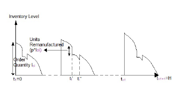Figure 1: Graphical representation of Inventory Model

Scenario 1: Desynchronized Model

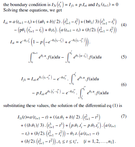the solution of the differential eq (2) is I_2i(t) =

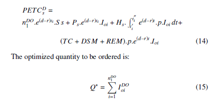
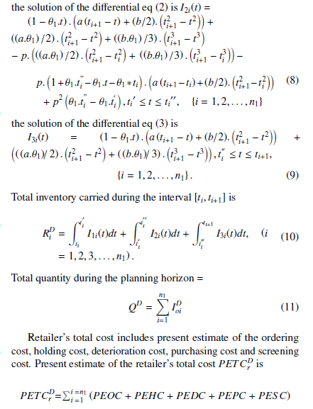Retailer’s total cost includes present estimate of the ordering cost, holding cost, deterioration cost, purchasing cost and screening cost. Present estimate of the retailer’s total cost PETC_r^D is

By determining the t_i⁰s, the green’s inventory model is optimized. Equation the first order derivative of the total cost to zero, the values are calculated.

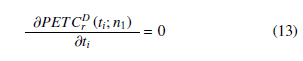The optimal solution so obtained by solving the above equation is n1DO, t0,t1DO, t2DO,…,tnDO1+1 = H,

With the existing replenishment schedule in the desynchronized model, the supplier determines his/her present estimate of the total cost by summing the setup cost,purchasing cost, holding cost, transportation cost, dissemmbly cost and the remaufacturing cost for the planning horizon H. The equation is as follows:

Scenario 2: Synchronized model with permissible delay

in the synchronized model supplier offers permissible delay to the retailer. On account of which the number of reordering cycle decreases,which further leads to a decrease in the setup cost of the supplier. With the new ordering plan, there is an increase in the cost for the retailer which the supplier compensates by distributing it through the parameter credit period rate.

For the new ordering plan n₂, the present estimate of the cost for the retailer is

The supplier compensates the retailer by adding the increase to his/her total cost and so the present estimate of the cost is

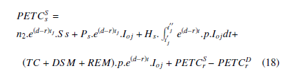The optimized value of the cost for the supplier PETC^S_s in the synchronized model is determined in the same way as done for the retailer PETC_r^D in the desynchronized model. n^SO₂ ,t₁^SO,t₂^SO,…,t_n^SO2₊₁ = H be the optimal solution for PETC^S_s .

The optimized ordering quantity in synchronized model is

QS = Pnj=SO2 1 IojSO

Equitable distribution of the extra cost incurred during synchronized model

For the retailer,the present estimate of the total cost in the synchronized model should be less than that in the desynchronized model, only then the new replenishment program is followed by the retailer.

where ρ is the credit period rate which is the distributing factor for the extra cost at the retailer’s end and the rate is same in all ordering intervals.

The credit period duration is given by:

MSj = ρtSOj+1 − tSOj

In the synchronized model,the supplier offers retailer credit for the minimum period.The credit period rate is kept minimum ρ_min to divide the benefits realized.The present estimate of his total cost in the synchronized model is then given by:

As supplier bears the additional cost borne at the retailer’s end, the credit period rate is maximum at his end ρ_max. His total cost in the synchronized model is given by the following equation:

The additional expenditure due to the replenishment plan of the synchronized model is fractioned on the basis of ρ¯, which is the average of the minimum and the maximum credit period rate. The present estimate of the net cost for both the retailer and the supplier is given by:

4.  Optimality Evaluation and Solution

The model is aimed at minimizing the total cost for the above cited two scenarios. The cycle time at which the cost is minimum is determined and the following theorem is verified with the help of the graphs.

Theorem 1: For any n₁,solution for the green supply chain EOQ model exists and is unique.

The convexity of the total cost can be seen through the following figures. Fig.2 plots the costs of retailer for the parameter SC = 4.5, and the value is minimum at the fourth cycle. The same is seen in Fig.3 for the supplier in the synchronized model where third cycle has a minimum value and the convexity of the cost is validated. The table values for the following figures is seen in Table 1 and Table 2 of the numerical example.

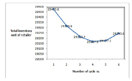Figure 2: Convexity of total cost for retailer at SC=4.5 in desynchronized system

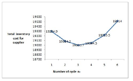Figure 3: Convexity of total cost for supplier at SC=4.5 in synchronized system

5. Algorithm

1. All the parameters are assigned the hypothetical values.
2. In the desynchronized structure, the optimal reordering point for the retailer is determined.
   • Taking t₁ = 0, n₁ = 1 and t₃ = H. Initializing t₂, and calculating it from equation (13).
   • Taking n₁ = 2.
   • From the values of t₁ and t₂ the value of t₃ is calculated from equation (13).
   • The optimal values of t_i⁰s is determined for every n₁.
   • For n₁= 1 and if PETC_r^D (n₁) < PETC_r^D (n₁ + 1), then PETC_r^D (n₁) = PETC_r^DO (n₁). Stop.
3. For n₁ ≥ 2 and if PETC_r^D (n₁) < PETC_r^D (n₁ − 1) and

             PETC_r^D (n₁)      <          PETC_r^D (n₁ + 1), then PETC_r^D (n₁)           =

PETC_r^DO (n₁) and stop or else let n₁ = n₁ + 1, and goto step 2(c).

4. n₁^DO = n₁ is the optimised cycle for both the retailer and the supplier in the desynchronized model.
5. PETC_r^DO, PETC_s^DO and Q^DO are determined from the respective equations.
6. In synchronized model,the optimal cycle time n^SO₂ , the present estimate of the cost for the retailer and the supplier PETC_r^SO and PETC^SO_s are calculated as done in steps from 2 to 4.
7. The values of ρ_min , ρ_max ,PETC_r^SOρ and PETC^SO_s ^ρ are determined from the respective equations.

5.1    Numerical Example

Hypothetical statistics is taken to validate the potency of the green inventory model.One principal parameter Screening Cost,SC is undertaken to observe the effects of changes in it on the optimal outcomes.

Example 1: a₁=20 items/year, b₁=5 items/year, θ₁ = 0.05 items/year, P_o = 4$/item,γ = 0.01,t₁ = 0,O_r = 25 $/purchase order, S _s = 30 $/arrangement, H = 4, P_s = 0.01 $/item, C_c = 2.5 $/item/year , H_o = 100 $/item/year, d = 0.1, r = 0.05, DC = 70 $/item, CT = 0.1, TC=0.01 $/item, REM=0.01 $/item, DSM=0.01

$/item.

Table 1: Inflated cost of retailer in the desynchronized model under green’s inventory system

SC		n1
	1	2	3
3	28568.6	28466.4	28422.2
3.75	28867.3	28821	28831.7
4.5	29167.3	29177.2	29243.6
SC		n1
	4	5	6
3	28568.6	28466.4	28422.2
3.75	28867.3	28821	28831.7
4.5	29167.3	29177.2	29243.6

The parameter of screening cost is further analyzed to study the impact of its changes on the green inventory model. Table 1 and Table 2 gives the total cost and the optimal ordering time period for both the retailer and the supplier in the desynchronized and the synchronized model respectively. Figure 2 and Figure 3 show the convexity of the cost.

Table 2: Inflated cost of supplier in the synchronized model under green’s inventory system

SC		n2
	1	2	3
3	19707.5	19299.4	19020.9
3.75	19474.8	19165.2	18984
4.5	19294.9	19084.3	19000.7
SC		n2
	4	5	6
3	18872.2	18853.3	18964.4
3.75	18931.1	19006.8	19211
4.5	19044.5	19215.5	19514

Table 3 shows that the optimal number of replenishment schedules after the synchronization diminishes when the screening cost increases. This signifies that the supplier will be benefited is he/she reduces the number of ordering cycles. To add on, the percentage in the cost savings of the supplier also increases when the parameter SC increases, which is agreeable as the supplier compensates for the increase in the cost of the retailer in the synchronized system. Moreover same trend in the cost savings is seen for the retailer also. the percentage cost savings increases for the retailer when SC increases, which will assure the retailer’s participation in the synchronized scheme.

Furthermore, the data also show that allowing for credit period, the optimal order quantity in the synchronized model is more than that as compared to the desynchronized model,thus raising the quantity ordered with reduced cycles.

Table 3: Percentage savings in cost for the retailer and the supplier in green’s inventory system

        4.5      29167.3      1195.08      4         117.79      0.273768

Synchronized system

SC	PETCrSOρ	PETCSOs ρ	nSO2	QSO
3	27730.2	1222.63	5	119.485
3.75	28131.3	828.518	4	119.485
4.5	28469.5	497.275	3	119.485

% Cost saving

SC	∆PETC PETCrDO	∆PETC PETCsDO
3	2.43485	36.144
3.75	2.3931	45.4288
4.5	2.39243	58.3899

6. Theoretical aspects in green inventory model on trade credit

Hypothesis 1: Permissible delay is negatively associated with the inflation rate.

To deal with the changes in the financial costs that incur due to the changing rate of inflation, organisations frequently alter the policy of trade credit. There is a decrease in the credit period to cope with the inflation. This study has been made by several researchers.The following table shows that as the rate of inflation increases, there is a decrease in the credit period rate. The data also reveals that although inflation is anticipated yet there is a realization of cost savings for both the retailer and the supplier in the green inventory model.

Table 4: Effect of change in rate of inflation on credit period rate

∆PETC r               ρ¯            DO PETCr	∆PETC PETCsDO
0.025 0.807762 2.30863	33.2966
0.05     0.728549 2.43486	36.1441
0.075 0.653612 2.55951	39.0887

Hypothesis 2: Permissible delay is negatively associated to the capital cost.

Supplier incurs extra cost due to permissible delay. However, both the retailer and the supplier at distinct rates can make financial investments. So with the increase in the capital cost, there is a reduction in the credit period rate. Furthermore,the percentage savings in the cost for the retailer and the supplier is not associated with the alterations in the capital cost.

Table 5: Effect of change in rate of Capital cost on credit period rate

∆PETC Cc ¯ρ                               DO PETCr	∆PETC PETCsDO
1.5 1.45327     2.4252	36.1042
3      0.728548 2.43485	36.144
4.5 0.485699 2.43485	36.144

Hypothesis 3: Credit period rate is negatively associated with the deterioration.

When the inventory of finished goods is perishable, there is a decrease in the revenue collected due to deterioration. For the deteriorated goods the time duration for permissible delay also decreases.The hypothesis is validated by the numerical example and the following table. To add in the validation for the hypothesis [33],[34] and [35] too derived the same result through the mathematical model in their research work.

Table 6: Effect of change in rate of deterioration on credit period rate

∆PETC θ1                       ρ¯            DO PETCr	∆PETC PETCsDO
0.0025 0.762206 2.26233	33.3653
0.005     0.728544 2.43483	36.144
0.0075 0.696866 2.70232	40.493

Hypothesis 4: Permissible delay is positively associated with the supplier’s set up cost.

There is an increase in the credit period rate when the parameter Ss increases. This guarantees that the supplier prolongs the permissible delay period to attain the benefit from synchronization. A majority of works by [36], [37], [33] predicted through their work, the attribution of the firm’s profitability with respect to the increase in the delayed time and the set up cost. There is percentage cost savings fruition for the supplier which enables him to extend credit period incentive to the retailer. The retailer too generates percentage savings in the cost,thereby motivational for him to accept the synchronization scheme.

Table 7: Effect of change in supplier’s set up cost on credit period rate

Ss	ρ¯	∆PETC PETCrDO	∆PETC PETCsDO
15	0.536511	1.38002	30.8952
30	0.728547	2.43485	36.144
45	0.931589	3.54378	39.4326

Hypothesis 5: The change in the optimal total cost of the retailer and the supplier is negatively associated with the parameter p, but permissible delay is positively associated with p.

With the high value of the inspection rate,the imperfect goods are quickly removed,thus reducing the cost of holding. The percentage savings is negatively associated as the goods removed decreases the time period of the revenue generation. The credit period increases as it takes time for the imperfect goods to be remanufactured and get again absorbed as demand in the greens inventory model, thus validating the hypothesis.

Table 8: Effect of change in the parameter p on credit period rate

p	ρ¯	∆PETC PETCrDO	∆PETC PETCsDO
0.375	0.694987	2.78661	41.9272
0.75	0.737651	2.64678	39.2901
1.125	0.778312	2.49702	36.6757

6.1     Managerial Insights

The logical implications for the hypothesis derived are firm and clear through the numerical considered and also through the work done by various prominent researchers. First, the association of the delayed cash time period with the rate of inflation is shown. This suggest that, the longer delay time should be squeezed to short time period on account of increase in the rate of inflation. Although to reach to long term conclusions, further study on other parameters associated should be done. This hypothesis highlights the significance of the supply chain process in optimising the inventory and the inventory related cost. Next in the supply chain process, the parameters as the capital cost, deterioration, set-up cost and price are studied with the delayed time. Thus modelling a concept of payment time delay with the manangement of inventory can help the firms to grab the untapped gains.

6.2     Senstivity analysis

Sensitivity analysis is carried on the green inventory model analyzing whether the formulated model is influenced by the alterations in the input parameters.We analyze the consequence of the alterations in the factors against the changes in the total cost of the retailer, supplier and the credit period rate. Every parameter is altered by -50%, -25%, 25% and 50%, of the initial cost taken in Example 1.

The table 9 shows that the change in the cost of the retailer and the supplier increases as demand increases which is agreeable. Also there is a decrease in the percentage change in the credit period with the increase in the demand.

Table 9: Analysis on demand variable ‘a’

                    ∆PETC_r^SOρ ∗ 100%            ∆PETC^SO_s ^ρ ∗ 100%           ∆ρ∗ 100%

value          PETC_rOSOρ                                      PETCSO_sOρ                                     ρ_O

0.5            -30.0024                         -29.83                             2.8461

0.75          -15.36                             -6.576                             15.2355

1.25          15.3233                           5.503                              -8.733

1.5            30.6353                           10.7837                           -15.479

The analysis on the holding cost of the supplier indicates that with the increase in the cost value the change in the cost of the supplier increases and also the rate of credit period increases.This implies that the supplier’s total cost is sensitive to the holding cost as shown in Table 10.

Table 10: Analysis on holding cost of supplier H_s

                    ∆PETC_r^SOρ ∗ 100%             ∆PETC^SO_s ^ρ ∗ 100%           ∆ρ∗ 100%

value          PETC_rOSOρ                                      PETCSO_sOρ                                     ρ_O

35	0.5753	-13.003	-15.219
52.5	0.2850	-6.449	-7.548
87.5	-0.2848	6.452	7.551
105	-0.5697	12.905	15.105

With the analysis done on the ordering cost of the retailer as in Table 11, it is evident that when the ordering size increases the total cost of the retailer increases. But there is a decrease in the cost of the supplier as the number of cycles decreases which is the synchronized model.

Table 11: Analysis on the Ordering cost O_r

                               SOρ                                                    SOρ

value ∆PETCPETC_rOSOrρ ∗ 100%        ∆PETCPETCSO_sOsρ ∗ 100%    ∆ρOρ∗ 100%

12.5	-0.8777	17.69	19.444
18.75	-0.444	8.96	9.851
31.25	1.110	-24.81	-27.772
37.5	1.849	-47.07	-48.271

When the parameters P_s and REM are examined,the data is recorded in Table 12 and Table 13. It is seen that with the increase in the purchasing cost and the remanufacturing cost, percentage change in the the total cost of the supplier also increases which is apparent. The supplier’s total cost is sensitive to these cost parameters. The credit period rate also increases wth the increase in these parameters. Although the retailer’s cost is less responsive to these cost parameters. With the increase in the credit period the retailer can invests the amount to generate gains.

Table 12: Analysis on the Purchasing cost of the supplier P_s

                     ∆PETC_r^SOρ ∗ 100%            ∆PETC^SO_s ^ρ ∗ 100%          ∆ρ∗ 100%

value            PETC_rOSOρ                                    PETCSO_sOρ                                    ρ_O

0.005	0.0093	-0.3012	-0.2619
0.0075	-0.000293	-0.0328	-0.00151
0.0125	0.000299	0.0327	0.00136
0.015	0.000594	0.0655	0.00283

Table 13: Analysis on the Remanufacturing cost of the supplier REM

                     ∆PETC_r^SOρ ∗ 100%            ∆PETC^SO_s ^ρ ∗ 100%          ∆ρ∗ 100%

value            PETC_rOSOρ                                    PETCSO_sOρ                                    ρ_O

0.005	0.0102	-0.2518	-0.2946
0.0075	0.0002	-0.0138	-0.0162
0.0125	-0.0001	0.0137	0.0160
0.015	-0.0003	0.0276	0.0322

7. Conclusion

The research demonstrates a synchronized supply chain with permissible delay under inflation in a greens inventory system. The model shows that the organizations can adopt for the green technology favouring the environment and can still realize cost savings. The study shows that the cost under inflation in the synchronized model is not more than the cost in the desynchronized model. The primary characteristic of the synchronized model is the credit period rate. It divides the extra cost incurred to the retailer on account of accepting the new ordering plan by the supplier and the extra cost incurred to the supplier on account of green’s technology of remanufacturing and recycling. The analysis of the model reveals that both the retailer and the supplier are able to generate financial benifits. Logical insights are proposed for the various parameters in this study.

Conflict of Interest

The authors declare no conflict of interest.

Acknowledgment:

The authors sincerely thank and appreciate the editor-in-chief and the anonymous reviewers who have considerably helped with their observations and insightful suggestions for the refinement of the paper.

1. Vikramjeet Singh, Seema Saxena, Rajesh Kumar Gupta, Nitin Kumar Mishra, and Pushpinder Singh. A supply chain model with deteriorating items under inflation. In 2018 4th International Conference on Computing Sciences (ICCS), pages 119–125. IEEE, 2018.
2. Michael W Toffel. End-of-life product recovery: Drivers, prior research, and fu- ture directions. In Conference on European Electronics Take-back Legislation: Impacts on Business Strategy and Global Trade. Citeseer, 2002.
3. David A Schrady. A deterministic inventory model for reparable items. Naval Research Logistics Quarterly, 14(3):391–398, 1967.
4. Maurice Bonney, Svetan Ratchev, and Idir Moualek. The changing relation- ship between production and inventory examined in a concurrent engineering context. International Journal of Production Economics, 81:243–254, 2003.
5.  Marisa MP de Brito. Managing reverse logistics or reversing logistics manage- ment? Number ERIM PhD Series; EPS-2004-035-LIS. 2004.
6.  Biswajit Sarkar, Waqas Ahmed, Seok-Beom Choi, and Muhammad Tayyab. Sustainable inventory management for environmental impact through partial backordering and multi-trade-credit-period. Sustainability, 10(12):4761, 2018.
7.  P. M. Ghare and G. F. Schrader. (1963) A Model for an Exponential Decaying Inventory. Journal of Industrial Engineering, 14, 238-243. J. Ind. Eng., 14: 238–243, 1963.
8.  Richard P Covert and George C Philip. An eoq model for items with weibull distribution deterioration. AIIE transactions, 5(4):323–326, 1973.
9.  Fred Raafat. Survey of literature on continuously deteriorating inventory models. Journal of the Operational Research society, 42(1):27–37, 1991.
10.  Hui-Ming Wee. Economic production lot size model for deteriorating items with partial back-ordering. Computers & Industrial Engineering, 24(3):449– 458, 1993.
11. H-M Wee and C-J Chung c. Optimising replenishment policy for an integrated production inventory deteriorating model considering green component-value design and remanufacturing. International Journal of Production Research, 47–1368, 2009.
12.  Kun-Jen Chung. An algorithm for an inventory model with inventory-level-dependent demand rate. Computers & Operations Research, 30(9):1311–1317, 2003.
13.  M Rameswari and R Uthayakumar. An integrated inventory model for de- teriorating items with price-dependent demand under two-level trade credit policy. International Journal of Systems Science: Operations & Logistics, 5 (3):253–267, 2018.
14. Karuppuchamy Annadurai. Integrated inventory model for deteriorating items with price-dependent demand under quantity-dependent trade credit. Interna- tional Journal of Manufacturing Engineering, 2013, 2013.
15.  Suresh Kumar Goyal. Economic order quantity under conditions of permissible delay in payments. Journal of the operational research society, 36(4):335–338, 1985.
16.  Kun-Jen Chung and Leopoldo Eduardo Ca´rdenas-Barro´n. The simplified so- lution procedure for deteriorating items under stock-dependent demand and two-level trade credit in the supply chain management. Applied Mathematical Modelling, 37(7):4653–4660, 2013.
17.  Biswajit Sarkar. An eoq model with delay in payments and time varying deterioration rate. Mathematical and Computer Modelling, 55(3-4):367–377, 2012.
18. T Sarkar, SK Ghosh, and KS Chaudhuri. An optimal inventory replenishment policy for a deteriorating item with time-quadratic demand and time-dependent partial backlogging with shortages in all cycles. Applied Mathematics and Computation, 218(18):9147–9155, 2012.
19.  Zhihong Wang and Shaofeng Liu. Supply chain coordination under trade credit and quantity discount with sales effort effects. Mathematical Problems in Engineering, 2018, 2018.
20.  Tsung-Te Lin and Jian-Hsin Chou. Trade credit and bank loan: Evidence from chinese firms. International Review of Economics & Finance, 36:17–29, 2015.
21.  Yong-Wu Zhou, Zong-Liang Wen, and Xiaoli Wu. A single-period inven- tory and payment model with partial trade credit. Computers & Industrial Engineering, 90:132–145, 2015.
22.  Brahima Coulibaly, Horacio Sapriza, and Andrei Zlate. Financial frictions, trade credit, and the 2008–09 global financial crisis. International Review of Economics & Finance, 26:25–38, 2013.
23.  Vikramjeet Singh, Nitin Kumar Mishra, Sanjay Mishra, Pushpinder Singh, and Seema Saxena. A green supply chain model for time quadratic inventory dependent demand and partially backlogging with weibull deterioration under the finite horizon. In AIP Conference Proceedings, volume 2080, page 060002. AIP Publishing, 2019.
24.  Brojeswar Pal. Optimal production model with quality sensitive market demand, partial backlogging and permissible delay in payment. RAIRO-Operations Research, 52(2):499–512, 2018.
25. JA Buzacott. Economic order quantities with inflation. Operational research quarterly, pages 553–558, 1975.
26.  Sh-Tyan Lo, Hui-Ming Wee, and Wen-Chang Huang. An integrated production- inventory model with imperfect production processes and weibull distribution deterioration under inflation. International Journal of Production Economics, 106(1):248–260, 2007.
27. Mohammadmahdi Alizadeh, Hamidreza Eskandari, S Mehdi Sajadifar, and Christopher D Geiger. Analyzing a stochastic inventory system for deteriorat- ing items with stochastic lead time using simulation modeling. In Proceedings of the Winter Simulation Conference, pages 1650–1662. Winter Simulation Conference, 2011.
28.  Maryam Ghoreishi, Gerhard-Wilhelm Weber, and Abolfazl Mirzazadeh. An inventory model for non-instantaneous deteriorating items with partial back- logging, permissible delay in payments, inflation-and selling price-dependent demand and customer returns. Annals of Operations Research, 226(1):221–238, 2015.
29.  Vikramjeet Singh, Seema Saxena, Pushpinder Singh, and Nitin Kumar Mishra. Replenishment policy for an inventory model under inflation. In AIP Confer- ence Proceedings, volume 1860, page 020035. AIP Publishing, 2017.
30.  Smita Rani, Rashid Ali, and Anchal Agarwal. Green supply chain inventory model for deteriorating items with variable demand under inflation. Interna- tional Journal of Business Forecasting and Marketing Intelligence, 3(1):50–77, 2017.
31.  Pushpinder Singh, Nitin Kumar Mishra, Manoj Kumar, Seema Saxena, and Vikramjeet Singh. Risk analysis of flood disaster based on similarity measures in picture fuzzy environment. Afrika Matematika, 29(7-8):1019–1038, 2018.
32.  Daniel Seifert, Ralf W Seifert, and Olov HD Isaksson. A test of inventory models with permissible delay in payment. International Journal of Production Research, 55(4):1117–1128, 2017.
33.  Abubakar Musa and Babangida Sani. Inventory ordering policies of delayed deteriorating items under permissible delay in payments. International Journal of Production Economics, 136(1):75–83, 2012.
34. Xiping Song and Xiaoqiang Cai. On optimal payment time for a retailer un- der permitted delay of payment by the wholesaler. International Journal of Production Economics, 103(1):246–251, 2006.
35.  YW Zhou and D Zhou. Determination of the optimal trade credit policy: a supplier-stackelberg model. Journal of the Operational Research Society, 64 (7):1030–1048, 2013.
36.  Jianwen Luo and Qinhong Zhang. Trade credit: A new mechanism to coordi-
37. nate supply chain. Operations Research Letters, 40(5):378–384, 2012.

(Click Here)

(Click Here)