1. Introduction

In inventory models, perishability is a physical property of inventories that results in the eventual expulsion of these goods from the system as waste [1]–[3]. In terms of social and commercial impact, studies on the management of perishables have prevailing importance. Products necessary to sustain human life, such as food and healthcare, possess this characteristic [4], [5]. In particular, the case of blood banks has received much attention from studies on perishable inventories. Due to the instability of supply and short validity of blood units, a precise and quantified means of managing these inventories are much needed [4], [6]. Blood banks are a strong example of how perishability as a product characteristic can complicate inventory systems, and can be used to generate insight on how other perishable products are best to be managed [6].

Perishability complicates the traditional inventory and supply chain models. The typical components of such models are profit and sustainability measures, capacity constraints, and demand distributions [7], [8]. However, policies that prove optimal for non-perishables are not necessarily optimal for perishables [5], [6]. In some models, perishability is represented as the deterioration of product quality [5], [9]. This can affect demand or the allowable pricing, thereby sharply differentiating the scenario described from inventory systems that do not differentiate between fresh and aged inventories. The transition of inventories from a state of salability to wastes is another differentiating factor. The production of wastes affects system capacity [10], [11], and any wastes generated may incur disposal costs [11], [12]. In this case, perishability affects key system constraints and parameters. Some studies on this subject have been dedicated to studying the differences between perishable and non-perishable systems. These have proven that the differences between perishables and non-perishables result in different optimal policies for each kind of inventory.

The majority of studies in this area are optimization models. From the models themselves, decisions on production quantity and product timing can be determined for a given set of parameters. In turn, managerial insights on managing inventory given similar parameters can be derived from the quantitative behavior of the variables. The optimization of inventory systems is a continuously growing body of research, with models growing in scale and complexity, or through the incorporation of new components such as technology enhancements [3], [13]. Aside from this, research efforts are also being invested in identifying the most efficient algorithms for the model [9], [14]. All in all, advancements in this area are geared towards achieving greater accuracy and numerical exactness. However, a weakness of this approach could be that the emphasis on these aspects of modelling shifts the focus away from insight-generation. While the models are becoming increasingly adept at describing specific scenarios, it may be noted that real inventory systems are constantly subject to external change. Thus, regardless of the level of exactness that is achieved by these models, its direct applicability to real systems will always be limited.

In response to these issues with current modeling approaches, applying the system dynamics methodology can augment these through (1) its applicability to large-scale systems which mathematical modeling may be inefficient for [15], (2) its emphasis on patterns of behavior over numerical exactness [16], [17], and (3) its limitation to constant system elements, as opposed to designing in response to external factors [18], [19]. The first two attributes make system dynamics apt for identifying key areas for solution implementation. Specifically, it can be used to identify the most influential variables in the system. This is insightful for future studies, which can delve more specifically in those areas. The third attribute aids in generating insight for recurrent managerial policies as opposed to period-specific decisions. These are more aligned with real managerial practices which, where rules and guidelines are favored to specific values.

In this study, the system dynamics (SD) methodology is applied to the case of perishable inventory systems. This is done for the purpose of demonstrating how the SD methodology can be applied in designing managerial guidelines, with proof that use of these guidelines will generate significant improvement for the system. As SD has already generated insights for general supply chain settings [20], [21], this study now investigates how perishability can alter the results, given that perishability has been proven to be a significant differentiating factor in previous studies [22]–[24]. Through its high-level perspective, the current study aims to identify impactful areas for solution development in the perishable inventory scenario. In this way, it can contribute to the area of study with suggestions for future studies focusing on these specific areas.

2. Literature Review

2.1. Inventory System Dynamics

There seems to be a limited research concerning inventory system dynamic (ISD) studies, thus there is potential to address multiple unexplored research gaps [19]. The challenge then is to find a purposeful gap to address, and justifying why system dynamics (SD) methodology would be more appropriate over methods that allow for more quantitative accuracy and optimization. In this respect, a review of the existing ISD studies is conducted to (1) learn the research objectives that prompted the use of SD, (2) understand how the ISD study relates to other inventory models using different methods, (3) understand how managerial and policy-making insights are derived from such studies, and (4) determine the main contribution of individual ISD studies.

In a literature review on SD applications in renewable energy supply chains, Saavedra 2018 observed that related studies seems to have objectives of either (1) improving understanding of the supply chain; or (2) developing modelling and simulation approaches. As a framework for understanding, SD is effective in depicting complex cause-and-effect chains and various sectors through its diagram-based modelling approach. From its diagramming methods alone, insight can be derived from the network of interrelationships between variables. On the other hand, as a simulation tool, the effectiveness of SD in providing insight is still being validated. This is due to its lack of quantitative accuracy and the lack of studies in this area.

Generally, a well-accepted method of applying SD is to use the diagramming approach to identify problematic areas, and apply sensitivity analysis to determine the most efficient area for solution [25]. This is the approach taken by studies seeking to apply the SD framework in a specific context. On the other hand, in studies that assess the methodology itself, SD has been coupled with various methods to augment its lack of numerical soundness, and the lack of perspective in other modeling approaches [19].

Given its frequent applications in sustainable supply chain models, there is often a part of SD studies that compares its methods with the likes of operations research and life cycle assessment (LCA), and validates that it can produce insights beyond those that can be derived from other modeling approaches. In comparing supply chain models using SD with those using other methodologies, Saavedra 2018 concluded that a major difference between SD and LCA is its focus on the behavioral patterns of variables within a model, such as the intermittency and variability of its values. On the other hand, the focus on LCA is on aggregate performance, such as the total volume of emissions [18].

The SD methodology also allows for a wide range of variables to be modeled and simulated efficiently, given its lack of numerical exactness. In a literature review, it was observed that most SD supply chain models had a macroscopic perspective consisting of economic and environmental impact. Next in quantity were SD studies with an inter-organizational scope, and last were studies with an intra-organizational scope. On the contrary, for operations research-based studies, the order from highest to lowest volume of publications is intra-organizational, inter-organizational and macroscopic [19]. This can alter the kinds of policies that may be developed and simulated using each method.

SD can be a means of extending optimized parameters into concrete policies, particularly in cases with multiple parameters of a different nature. Song 2018 created a model to simulate the application of optimized parameters for technology, environment, energy and economy in a system where they are interrelated. These parameters were derived using data envelopment analysis (DEA), which augments the lack of numerical accuracy in most SD models. SD then strengthens the policy-making approach by highlighting the physical relationship between variables.

Scenario analysis, such as applying different parameters to represent different cases, is a quick means of validating the model’s logic and policy development. In validation, it allows for multiple real-life case parameters to be applied to prove the validity of the causal relationships and the completeness of the model. In policy-making, a number of alternative solutions can also be generated and simulated, by shifting model parameters [18].

Overall, SD studies have contributed to the field of study with insight for how certain resources can be managed with optimal results [25]; knowledge on the opportunities and limitations of simulation methods [18]; and the creation of hybrid models combining SD with more math-based methodologies [19].

2.2. Perishable Inventory Systems

Perishable Inventory Systems (PIS) have received much attention in literature as early as the 1990s, up until recent time [5]. Earlier studies simply sought to incorporate ‘perishability’ as an attribute of inventory. Nonetheless, more recent studies seek to determine the kinds of managerial strategies and policies that may be applied to perishable inventories [2], [26]

In a literature review conducted in [5], studies from 2012 to 2015 were segregated according to the different policies being implemented in each study. It was found that the top policies being studied during that period were (1) credit and payment policies, (2) supply chain information sharing, and (3) pricing and markdown problems. There were notably few studies on the use of the introduction of advanced monitoring technology, and on classic issuance policies (i.e. FIFO, LIFO).

Since then, there has been an increase in models on the integration and use of monitoring technology in perishable inventory systems. [6] have introduced the use of RFID technology in monitoring of unit age and cost to the dual-sourcing problem for perishables. This was evaluated against fixed and exponential product lifetime scenarios, to gain insight on specific potential applications for this strategy. More recently, [3] have developed an IoT-based model for monitoring perishables in shared storage. Given the potential for cross-perishability, which refers to the increase or decrease in deterioration rate resulting from shared storage, information monitoring in this manner could then allow for lowering of deterioration costs, inventory level, and quality loss for the system. On a two-stage optimization model for pricing and replenishment of PIS, the recommended extension is also the incorporation of RFID and point-of-sales data in decision-making [7].

It seems to be reasonable for research to progress in this direction given the rise of Industry 4.0 [27], [28]. However, the implementation of advanced systems, similar to the aforementioned, are still dependent on fundamental decisions in inventory management. This is evidenced by the way that these technologies are modeled in conjunction with inventory management policies from classic literature [29]. Yet, these policies are still among the top policies being studied from 2012 to 2015, as identified by [5].

Over the years, there have been few changes to the performance functions used for perishable inventory models which enable ease of comparison. Financial measures such as profit and cost are still used in almost every PIS study. The percentage of profit growth or cost reductions resulting from the implementation of certain policies is typically used as the measure of performance in these cases [4], [6], [26]. Profit can be affected by perishability through the decline of demand alongside quality [30]. It can also manifest as disposal costs [2], [8] and wastes [7].

Wastes differ from financial measures as they are a physical outcome of the PIS policy. By quantifying waste production, a model can also be assessed for its sustainability [10], [11]. The minimization of waste, separate from its contributions to cost, is used as an objective in a number of studies [5]. In this way, the model can differentiate between financial and physical outcomes, given that the volume of wastes would not always be economically relevant in all cases.

Another physical outcome of PIS policy is the service level, or the ability to meet customer demand [28]. In the model of [7], service level is the probability of stockout in the replenishment cycle resulting from the policy. Monitoring the service level of PIS prevents over-emphasis on cost efficiency, in a more tangible way than revenues. Aside from this, the model of [4] has made use of the average age of inventories being sold, to represent the quality of the products.

The perishable nature of inventories in PIS is represented as a finite lifetime. This leads to wastes at the end of the product lifetime [11], [12], and declining demand over time for a specific unit [5], [9], [31]. In most PIS models, a scenario analysis is conducted for various rates of deterioration. Generally, the higher the deterioration rate, the greater the amount of waste [7]. However, this can also vary depending on the stochastic distribution of a product’s lifetime, and the kind of policy being implemented. The model of [6] demonstrates that dual-sourcing can produce greater cost savings in cases where lifetime is fixed with a shorter average, and when lifetime is exponentially distributed with a longer average.

Generally, a number of policies have proven effective in managing PIS, with immediate improvements in cost and material efficiency. Optimization models demonstrate how such policies can be applied with optimal results for a given set of parameters. However, the existing methodologies have proven to be inefficient for policy-to-policy comparison, given the variability in model structures and sensitivity to parameters. Thus, the basis of determining best practices based on the existing studies could still be improved.

2.3. FIFO and LIFO Issuance Policies

Issuance policies are an integral part of an inventory management problem. In general, the parameters under study in such a problem are pricing, inventory costs, and deterioration rate [7], [32]. These parameters are present in almost all studies and are used to evaluate specific policies being applied, or intended for application, on real inventory systems. These policies can include issuance policies (i.e. FIFO and LIFO), which relate to the order at which goods of the same kind at different ages are dispatched to the customer. Based on the review of Janssen (2016), issuance policies appear to be an overlooked area in literature. However, based on the current review that was conducted, it seems that most studies include issuance policies as a parameter, instead of treating it as a focus of the study. The review of literature in this area is thus segmented in two ways: (1) studies considering issuance policies as a parameter, and (2) studies explicitly focused on evaluating or identifying optimal issuance policies.

Using a policy as a parameter means that it can be changed to allow the analyst to see various scenarios. [23] sought to determine how the centralization of inventory could be beneficial in managing a perishable supply network. Specifically, the case under consideration was a blood supply chain with inventory located at a single blood bank and being supplied to multiple hospitals. FIFO was explicitly modeled for this case, as this is the standard for inventories in the healthcare service industry. [10] adapted a modeling and simulation analysis methodology determine the impact of a closing day constraint for the inventory of stores. The objective of the study was to determine if the existence of a closing day would lead to more aged inventory as closing day approach, as is the case in real grocery store inventories. It was found that the closing day constraint did result in simulated behavior being closer to the real behavior of inventories. In another study, [11] assessed the quantitative impact of micro-periodic inventory management policies, for how these may potentially improve costs and waste production. Under this approach, a single day was broken into morning, midday, afternoon and evening periods. This likewise made use of a mixed FIFO and LIFO approach. It was found that costs were reduced significantly from micro-periodic management, as compared to daily planning.

One reason why a mixed approach is taken in most studies is so that the exact impact of each policy will not have to be considered. This recognizes that there are, in fact, real differences between the effects of applying each policy, particularly on perishables. The models that explicitly analyze the issuance policies seek to determine what these effects are and how they can be managed most effectively to meet the goals of the system. [12] compared the viability of FIFO and LIFO for managing perishable inventories using a modified Economic Manufacturing Quantity. Said model was modified to give consideration for fixed order quantity and joint ordering policies. This revealed that LIFO could prove optimal under linearly decreasing price structures. This finding is relevant given that it is generally accepted that FIFO has superior performance on perishables [19], [23].

In most cases, issuance policies are modeled as a two-warehouse problem. Under LIFO, the first inventories to be sold would come from the rented warehouse; while under FIFO, the first sales are taken from the owned warehouse. A model for this problem was developed by [32], who assessed each issuance policy for its overall costs, given deterioration and holding costs. It was found that FIFO was less expensive when the cost parameters were lower for the owned warehouse than in the rented warehouse. As this is the case for most entities, it may be concluded that the study recommends FIFO under LIFO given the parameters that were considered. [9] extends the study of issuance policies for two-warehouse inventory systems to the use of modified FIFO (MFIFO) and modified LIFO (MLIFO) policies. Under the MFIFO rule, the FIFO rule is followed as far as the inventory in demand is available. When unavailable, the backorder gets assigned to the lowest priority level in the next period [28]. The model was structured in such a way that allowed for easy comparison between policies by relaxing a few constraints. It was found that when deterioration rate was different between the rented and owned warehouses, holding cost could make a significant difference in the optimality of each policy.

MFIFO and MLIFO are already evolutions of the existing issuance policies. It is understood that FIFO and LIFO each have weaknesses, and thus improvements can be made in their exact rules. [31] proposed the development of a new issuance policy entitled Allowance-in-Fraction-Out which has specific rules for when to apply FIFO and LIFO. This is likewise applied to the two-warehouse inventory problem, wherein the decision to switch is based on the fraction of rented warehouse inventory to owned warehouse inventory. Across various cases of deteriorating behavior, value of information, and perishability, it was found that the mixed method could have benefits in transportation costs and the occurrence of sub-replenishments.

In recent literature, most studies treat issuance policies as a parameter. Moreover, most studies assume a mixed issuance policy structure to protect the model from the effects of using any specific policy. However, this suggests that inventory will be taken randomly from a company, which is understandably not the case in inventory systems. The most advanced study in this area seeks to determine the appropriate rules for using FIFO and LIFO, and managing their negative repercussions. This would imply that further study is needed of the explicit behaviors of FIFO and LIFO to determine how they may be managed productively.

3. Methodology

In this study, the system dynamics (SD) methodology is used to model a perishable inventory model, and simulate the application of certain policies and methods. This method is efficient for analyzing patterns of behavior, as it emphasizes long-term patterns over quantitative accuracy [16], [17]. It is also efficient in expanding the scope of a model to encompass all variables that could have significant feedbacks on the key variables under study [20]. SD emphasizes the importance of feedbacks in a system, showing how the system’s behavior is actually the result of these internal feedbacks, and not external factors [16]. In problem solving, this maintains the focus on constant factors, rather than externalities which may or may not be present. In this way, the SD methodology is well-suited for evaluating policies in the long-term, and managing any negative repercussions that may result from their application.

The SD framework is applied with the intention of designing policies that will improve the sustainability and quality goals of the system. Most perishable inventory models attempt to address sustainability goals by having waste minimization as one of its objectives [30], [33]. The connection of waste minimization to sustainability implies that through waste reduction, resource consumption is also reduced. On the other hand, quality goals can be met in terms of age-based quality, by minimizing the time a unit spends in the system from production to sale [4]. Age or, conversely, freshness is an apt representation of quality for perishables given the fact that (1) perishables are typically fast-moving consumer goods which vary little from unit to unit, and (2) perishables will definitely degrade in some way over time, making age a significant component of quality, even if it is not the sole component.

The SD methodology classifies variables as stock, flow, auxiliary or exogenous based on their role in the model. Stock variables accumulate over time based on previous values; flow variables represent this rate of accumulation; auxiliaries serve as the transition of stocks to flows; and exogenous variables are parameters whose values are externally determined. A discussion of how the variables were classified, and of their respective equations is given in Section 3.1. Following this, the variables determined in Section 3.1 are organized in a causal loop diagram in Section 3.2. This represents the relationship of the variables in an enclosed system. The variables and loop structure are then integrated in a stock-flow model for simulation and analysis in Section 3.3.

3.1.  Variables Definition

Stock variables are those which increase or decrease in relation to their value in a previous period. This can be used to represent inventory levels which physically change over time. In this model, inventory is divided into two categories based on age. Hence, there is a variable representing Fresh Finished Goods Inventory (FFGI) and Previous Finished Goods Inventory (PFGI) respectively, as levels. By logic, FFGI is a function of production, sales, and leftover inventory in the current period (t). Since it is not an option to dispose freshly-produced goods in this model, there is no difference between the equation for FFGI in the perishables and non-perishables case.

FFGI(t) = FFGI(t-1) + Prod.(t) – Sold F. Inv.(t) – Held Inv.(t)

(1)

PFGI represents inventory carried over from previous periods. In the perishable’s scenario, a fraction of inventory becomes waste at the end of each period. Mathematically, these differences between the perishables and non-perishables case are given in equations 2 and 3 respectively.

PFGI(t) = PFGI(t-1) + Held Inv(t) – Sold P. Inv(t) – Wastes(t)	(2)
PFGI(t) = PFGI(t-1) + Held Inv(t) – Sold P. Inv(t)	(3)

Aside from variables that physically change in value, stock variables are also apt for representing human cognition in system dynamics models. Cognition is influenced by the occurrence or lack thereof of certain events. In consequence, these strengthen or weaken a certain idea, which in turn produces reactions affecting the other variables in the system. Such variables are usually not included in modeling as there is no definite metric to represent them. However, the soft emphasis on numerical accuracy in system dynamics allows for such variables to bear the same weight as tangible variables (i.e. inventory, cashflow).

In this model, there are two cognition variables, both represented as ‘perception’. One of these is Perceived Quality (PQ), representing the customer’s flawed knowledge on the actual quality of goods produced by the producer. System dynamics recognizes the feedback delay in perception of performance, which results in there appearing to be no effect despite efforts toward improvement. PQ changes by a positive or negative value, depending on whether the quality in recent periods has been good or bad. However, PQ itself will always be a normalized value as the change happens in relation to previous values of PQ. Conversely, Perceived Demand (PD) represents the producer’s flawed knowledge on the actual volume of customer demand. In real applications, this would represent the degree of error in demand forecasts [34]. Likewise with PQ, PD changes by a positive or negative value depending on the recent demand values.

The change in the value of stock variables at each period is defined as a flow variable. A stock can have inflows that add to its value, and outflows that reduce its value. In the case of FFGI, the inflow rate is Production (Prod), while the outflow rates are Held Inventory (Held Inv) and Sold Fresh Inventory (Sold F. Inv). Prod is based on the value of PD, which represents the use of forecasts in deciding on production quantities [32], [35].

Prod(t) = PD(t)

(4)

Held Inv is equal to the current value of FFGI, as all fresh inventory that is not sold will be carried over to the next period as PFGI. Held Inv represents the transition of FFGI into PFGI by being an outflow of the former into the latter. The also represents the aging of products in the system. In essence, there are only two age classes of goods–fresh and previous. While this may not capture the exact age of the inventory pieces, it is nonetheless sufficient to show the impact of FIFO and LIFO. Further segmentation by age group may further complicate the model without generating additional insight to compensate for the effort.

Held Inv(t) = FFGI(t)

(5)

FFGI and PFGI each have outflows in the form of sales, and the equations for these vary between the FIFO and LIFO cases given that the former prioritizes selling PFGI while the latter prioritizes selling FFGI [Parlar et al, 2011]. These are Sold Fresh Inventory (Sold F. Inv) and Sold Previous Inventory (Sold P. Inv). Mathematically, the prioritized inventory class is directly influenced by Customer Demand (Cust Dem), while the deprioritized class is a function of the sales for the prioritized class. The equations for the FIFO case are given in equations 6 and 7; and those for LIFO are given in equations 8 and 9.

Sold F. Inv(t) = MIN(MAX(Cust Dem(t) – Sold P. Inv(t), 0), FFGI(t))	(6)
Sold P. Inv(t) = MIN(Cust Dem(t), PFGI(t))	(7)
Sold F. Inv(t) = MIN(Cust Dem(t), FFGI(t))	(8)
Sold P. Inv(t) = MIN(MAX(Cust Dem(t) – Sold F. Inv(t), 0), PFGI(t))	(9)

For PFGI, there is an additional outflow in the form of Wastes. This variable is only present in the perishables case, as inventory can only be accumulated in the case of non-perishables. The variable Wastes is a function of the residual PFGI and a given rate of deterioration:

Wastes(t) = (PFGI(t) – Sold P. Inv(t)) / DelayP

(10)

For the cognition variables Perceived Demand and Perceived Quality, it was previously mentioned that the change could be positive or negative depending on the recent values of the perceived information. These changes are the flow variables Change in Perceived Demand (CIPD) and Change in Perceived Quality (CIPQ). Mathematically, a positive change would result if the current value is greater than the perceived value, and a negative change if otherwise. In effect, the current values are normalized against previous values. A feedback delay is used to represent the limited influence on current values against long-standing perception. In equation form:

CIPD(t) = (QOGS(t) – PQ(t)) / DelayPQ	(11)
CIPQ(t) = (Cust Dem(t) – PD(t)) / DelayPD	(12)

Aside from stock and flow variables, a system dynamics model contains auxiliary variables. These are components of flow variables. It can serve as a means of breaking down potentially-complex equations for flows, both for ease of understanding and to highlight the behavior of specific components. Auxiliaries are derived from the behaviors of stock variables, and can link these to flows in the model. Unlike stock variables they are not a function of their previous value. While they do not change the overall system behavior, they are nonetheless important for clarity in representation.

The model contains three auxiliary variables: Quality Multiplier (QM), Customer Demand (Cust Dem), and Quality of Goods Sold (QOGS). QM is an example of an auxiliary that exists for ease of understanding. Its value is equal to the value of Perceived Quality (PQ), yet the conversion is made to show the logic in making PQ part of the function of Cust Dem. Hence:

QM(t) = PQ(t)

(13)

Cust Dem is a function of two variables, QM and a randomized demand value that is exogenous to the system (Natural Range of Customer Demand, NRCD). In effect, the perception of good quality positively influences demand by a margin, while the perception of poor quality has an inverse effect. As indicated by its usage in the previous equations, customer demand is the actual amount of purchases made by the customer in a single period. This consequently affects the sales variables, Sold Fresh Inventory and Sold Previous Inventory. The equation for this variable is given as:

Cust Dem = NRCD * QM(t)

(14)

QOGS represents the quality of goods sold for a current period. In this model, the quality of the perishable product is solely based on freshness. Its value is derived from the amount of Sold Fresh Inventory (Sold F. Inv) in relation to Customer Demand (Cust Dem). Higher proportions of Sold F. Inv in Cust Dem would thus equate to better quality. As information on the quality of the producer’s goods is transmitted to the customer through sales, QOGS has a direct but gradual influence on PQ [30], [36].

QOGS(t) = 1 – Sold P. Inv(t) / Cust Dem(t)

(15)

The variables that are not directly influenced by any variable in the model are exogenous variables. The belief that the system’s behavior is primarily influenced by the feedbacks between its endogenous variables, rather than exogenous variables, are at the core of the system dynamics methodology. Hence, exogenous variables are typically represented by constant parameters, as proof that their value is of minor significance to the system’s behavior.

Feedback delays are a common example of an exogenous variable. These represent delays in the transmission of information across the system. In equation form, these are variables that limit the flow of information to a cognition variable. In this model, these delays exist in the flow variables for Perceived Quality and Perceived Demand, as Delay in Perception of Quality (DelayPQ) and Delay in Perception of Demand (DelayPD). Physical delays are another common exogenous variable, representing rates of transition from one state to another. In this model, the physical delay is the Delay in Perishing (DelayP). This delays the transition of inventory into wastes, according to a supposed validity period.

An exogenous variable is also used to represent additional sectors of the system that can be simplified for ease of analysis. This can be done when the variables included in that sector are not explicitly being analyzed. In this model, the Customer Demand (Cust Dem) is understandably an outcome of Perceived Quality. Yet, it is also influenced by the availability of other options in the market; the demand of the customer’s own customer; and numerous other factors depending on the specific case and scenario. In effect, Cust Dem will have a degree of variability due to these other variables. To represent this, a Natural Range of Customer Demand variable is introduced as a random variable with a given range.

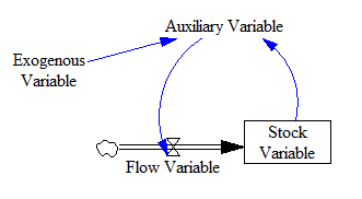Figure 1: Basic Structure of a System Dynamics Model.

3.2. Interactions Between Endogenous Variables

The greatest differentiating factor of the SD methodology is that it organizes variables into feedback loops. This follows the principle that a system’s behavior is influenced more by the system’s internal reactions than any external factor. A visual representation of the role of each kind of variable in a feedback loop is given in Figure 1. All loops include at least one stock variable, which shows how the current outcomes of a system result from behavior in a previous period. This progression of cause and effect leading from past to current behavior is demonstrated through a progression of auxiliary variables. It is shown in Figure 1 that auxiliary variables are the link from stock variables to flow variables, which mathematically means that the past values of a variable would change its next-period values. Finally, the exogenous variables are externally-determined and not influenced by any other variable in the system. Hence, there is no feedback leading to an exogenous variable.

To demonstrate the cause-and-effect relationships in a SD model, variables are arranged in causal loops without differentiation between variables. The purpose of this is to emphasize the feedbacks within the system prior to explicit modeling. In developing the causal loop diagrams for this study, it became apparent that there would be different causal loops for the FIFO and LIFO cases respectively, due to the difference in inventory type affected by sales. Specifically, demand directly impacts aged inventory in the FIFO case, and fresh inventory in the LIFO case. Aside from this, both cases have the same loops, representing a common PIS structure to enable comparison.

In PIS models, demand changes based on the age of inventory given the fact the that goods are deteriorating over time [5], [9]. In this model, a quality variable determined by age is positively linked to demand, meaning that demand will increase as quality improves. Quality is positively affected by the quantity of fresh inventory, and negatively affected by the quantity of aged inventory. This is how the reduction in demand caused by low-quality or aged goods is interpreted in the model. The resulting demand has a delayed impact on production, representing how demand from previous periods can determine production levels in the coming periods through forecasts. Production quantities then add to the level of fresh inventory, and fresh inventory becomes aged inventory, by natural progression [4], [11], [37].

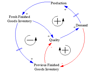Figure 2: Causal Loop Diagram for FIFO Scenario.

The amount of positive or negative relationships in a feedback loop determine the ‘positivity’ or ‘negativity’ of that loop. Even numbers of negative relationships create a positive loop, which prompts positive exponential growth in the variables involved. Odd numbers create a negative loop with negative exponential growth. In system dynamics, systems are understood to be composed of these positive or negative loops, which balance each other out. Following this perspective, the LIFO scenario is more balanced than the FIFO scenario, as it contains equal amounts of positive or negative loops. This suggests that behavior is more consistent under the LIFO scenario, than the FIFO scenario.

Figure 3: Causal Loop Diagram for LIFO Scenario.

3.3. Simulation Model Development

Using VensimPLE software, a system dynamics (SD) model was developed to simulate the postulated behaviors of each variable and analyze their interactions. The general form of the SD model is shown in Figure 4. This shows the variables identified in Section 3.1 in their proper form, and arranged in the feedback loops derived in Section 3.2. There are three major sections in the model: (1) the physical inventory system, which is also the main problem variable under study, (2) the perception of quality, representing the impact of the physical system on human receptors, and (3) the perception of demand, representing the human decisions which govern the physical system. These form a single loop that determines the behavior of the system.

The model parameters are feedback delays, which can be adjusted to represent various scenarios. The Delay in Perishing represents the validity period of the goods, which can vary depending on the nature of the goods. In PIS for blood banks, this parameter strongly impacts system behavior given the brief and stringent validity period of the inventory [23]. For disaster relief operations where goods are hardier, the impact of this parameter is less strong, given that the goods are practically non-perishable [2]. For the same reason, there are few disaster relief supply chain studies which consider waste and disposal.

The Delay in Perceived Quality represents how evident differences in quality may be to the customer. Smaller batch sizes and proximity to the end-customer can equate to shorter delays. In retail settings, which have this characteristic, demand is typically a function of quality [11]. On the other hand, upstream suppliers consider perishability in terms of waste and disposal costs, as opposed to impact on demand [23], [28].

Figure 4: Structure of Inventory System.

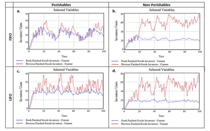Figure 5: Simulated Fresh and Aged Inventory Levels.

The Delay in Perceived Demand represents inaccuracies in the forecasting techniques with regards to real demand. There are countless studies on forecasting techniques and replenishment policies, and each have proven effective in specific contexts and following specific demand distributions. In such cases, the policies are evaluated by the resulting service level [4], [7]. The current model extends this to examine the reactions between the performance of the policy and other components of the system.

Following the structure in Figure 4, four models were created for each of the following scenarios: (1) FIFO applied to perishables, (2) FIFO applied to non-perishables, (3) LIFO applied to perishables, and (4) LIFO applied to non-perishables. The main difference between the perishables and non-perishables scenarios is the lack of a Waste outflow for aged non-perishable inventories. In this case, the only possible outflow is through sales. Given that the emphasis of this study is on perishable inventories, the policies that may trigger the disposal of non-perishables are not considered.

By logic, FIFO and LIFO differ based on the priority of inventories to be sold. These differences were given in equation form in Section 3.1 and in diagram form in Section 3.2. It is necessary to generate a different model to represent each case given that the feedback relationships differ. Hence, this is not a case of merely adjusting parameters to represent a case, but making adjustments to the model parameter. Aside from priority of sales, the structure of the model given in Figure 4 is maintained for all versions, to allow for the results to be comparable with one another. The simulation results depict values for the behavior of variables over time. This is analyzed in graphical form to assess the model for patterns and identify areas for problem-solving.

4. Simulation Results

All inventory models have the objective of minimizing inventory levels, whether directly or indirectly. In optimization models, inventory levels are often linked to cost objectives through holding costs and disposal costs [15], [35]. In this way, minimal inventory levels becomes the most economic scenario for an inventory system. In simulation methodologies, inventory is physically monitored with the unstated understanding that it affects other performance indicators, such as cost and wastage [5], [7]. The system dynamics methodology is aligned with this perspective. This study likewise monitors physical inventory levels as a performance measure, and evaluates its effect on outcome and quality.

As mentioned in Section 3.1, the perishable aspect of inventory is modelled by the transition of goods from a fresh state (Fresh Finished Goods Inventory) to an aged state (Previous Finished Goods Inventory). The model differentiates between inventory in only two ways, fresh and aged, based on their impact on the system. The system dynamics methodology is an efficient means of monitoring and analyzing such variables for this purpose. In mathematical models, inventory is represented in a very exact manner, indexed by time of production and sale [28], [31]. This can take the focus away from the more important implications of inventory.

Four scenarios are simulated: FIFO applied to Perishables, FIFO applied to Non-Perishables, LIFO applied to Perishables, and LIFO applied to Non-Perishables. Each scenario is evaluated by its resulting inventory level. The analysis can be segmented into three parts: (1) A comparison between the Perishables and Non-Perishables scenarios for logic-checking, (2) A comparison of the FIFO and LIFO scenarios for policy evaluation, and (3) Determining the optimal issuance policy to apply to perishable inventories.

4.1. Comparison of Perishables and Non-Perishables Scenarios

In Figure 5, sections a and c contain the simulated inventory levels for the perishables scenario, while sections b and d contain the results for non-perishables. In all cases, inventory levels exhibit oscillating behavior which is aligned with the behavior being demonstrated in other inventory models and supply chain industry studies [36]. The perishables and non-perishables scenarios differ in the long-term trend being demonstrated by inventory under each case. Under the non-perishables scenario, inventories exhibit an upwards trend, indicating the tendency for inventories to accumulate. Under the perishables scenario, inventory levels are stable in the sense that they exhibit no upwards or downwards trend. The volume of inventory in the perishables scenario is naturally regulated by the potential for wastes, which prevents accumulation. On the other hand, there is no negative feedback to control the volume of inventories in the non-perishables scenario, resulting in accumulation.

The simulated behavior for non-perishables is aligned with the behavior of most forecast-based non-perishable inventory systems. There is evidence to support this in the management of mechanical parts inventory, which has a large amount of excess [38], [39]. The accumulation may also be attributed to the fact that production quantity was based solely on sales forecasts, without any regard for current inventories. This mimics decision-making for perishables more closely. Since goods manufactured in one period do not have the same external value as goods manufactured in a different period, past inventory cannot be fully utilized to supply current demand. Therefore, decision-making parameters such as current inventory and safety stock generally carry more weight in models for non-perishable inventories.

The simulated behavior for perishable inventories follows the behavior of traditional inventory models (e.g. EOQ), which oscillate without any positive or negative trend. Inventory accumulates because of inaccuracies in forecast. Yet, because a fraction of perishable inventories become waste at the end of each period, inventories cannot accumulate. Instead, excess inventory from inaccuracies in in forecasting eventually leave the system as waste. This is not favorable given that the amount of inventory that become Wastes are just excess in a different form. It may only be said that inventory is more effectively-handled under the perishable scenario if the volume of its Wastes is not increasing in the same way excess inventory does for non-perishables. The simulated behaviors for waste, although oscillating, exhibit no increasing trend (see Figure 6). For these reasons, it may be concluded that perishable inventories do not have as strong of a tendency towards overproduction.

It may be concluded based on the simulated results for Previous Finished Goods Inventory that the main issue in the management of perishable inventory is not preventing surpluses and shortages. Under common inventory management policies, perishability as a product characteristic results in an inventory system that is less

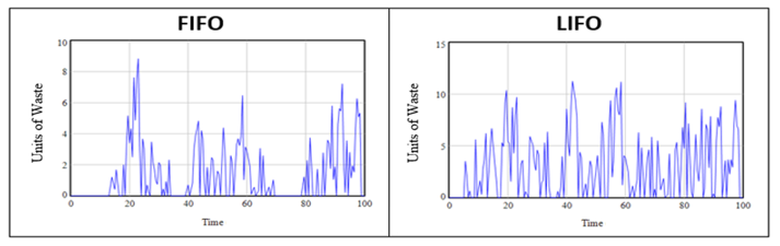Figure 6: Comparison of Waste Production for FIFO and LIFO.

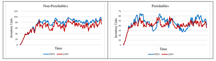Figure 7: Comparison of Aggregate Inventory Levels.

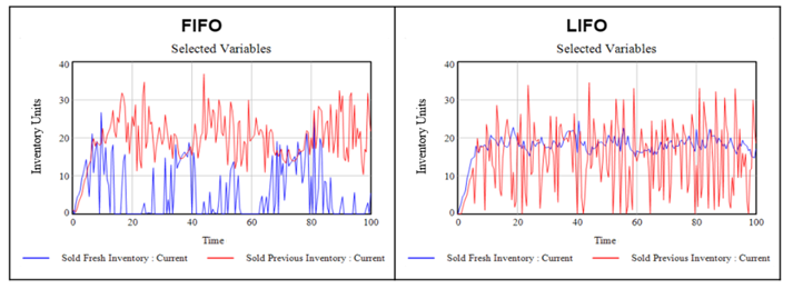Figure 8: Comparison of Sales for FIFO and LIFO.

prone to such outcomes. Inventory models with the objective of determining an optimal stockout level could thus be redundant, or even counterproductive to the system’s natural ability to regulate itself. On the other hand, the system could benefit from the minimization of its peak inventory levels, or all-around variability.

As the simulated behaviors follow the trend described by real industry data and by literature, the ensuing analysis can be deemed valid. A comparison may now be conducted between the FIFO and LIFO policies given the system structure. Based on the simulated values in Figure 5, it is apparent that the choice of issuance policy hardly makes a difference on inventory levels. On the other hand, there are clear differences between the FIFO and LIFO scenarios in the perishables case.

4.2. Comparison of FIFO and LIFO Scenarios

Generally, inventory levels are higher under the FIFO case. This is true for both the non-perishables and perishables cases. Figure 7 shows that in, the non-perishables case, inventory levels exhibit the same upwards trend. Yet, once the values stabilize, the FIFO case will begin to exhibit consistently higher inventory levels. Its highest point and lowest point upon stabilization are higher than inventory at any point in time under LIFO. This is different from the case of perishables, where inventory levels have higher maximum peaks under FIFO but also lower LIFO peaks. However, based on the simulations, it would appear that FIFO exhibits higher inventory levels more often than it exhibits lower inventory levels.

The higher inventories under FIFO may be attributed to the extent of feedback delay between production and demand. In the causal loop diagrams in Figure 2, there are multiple delays between Fresh Finished Goods Inventory and Demand under FIFO. This signifies that there are multiple delays between demand and production for forecasts based on it are actually sold. Hence, there is a higher propensity for overproduction or underproduction. In these cases, the problem is leaning towards overproduction given that current inventories are not considered in deciding on the quantity to produce in the next period.

Based on the review of studies on PIS, there are more models were FIFO proved to be optimal than otherwise. These models are optimization models with the primary objective of minimizing costs. The potential for waste production is incorporated in the form of disposal costs or deterioration costs, which align the sustainability and economic objectives for the system. It is understandable for FIFO to be optimal following this perspective, as FIFO results in the lower minimum inventory values. However, in actual inventory systems, stable inventories are preferred over fluctuations.

In literature, the case where LIFO proved to be optimal was the case where prices decreased linearly for each period that the inventory unit remained in the system. This would suggest that when quality affects revenues, LIFO becomes preferable. This is because the profit earned per unit would be more consistent. The key benefit to be derived from LIFO is consistency. In this model, quality affects revenues by acting as a multiplier to demand. Results showed that inventory levels were less variable for both perishables and non-perishables, which aligns with the suppositions from previous studies that LIFO can result in greater consistency.

4.3. Evaluation of FIFO and LIFO Applied to Perishables

For perishables, product quality is partially determined by the age of inventories. Hence, the volume of fresh and aged inventories can have an impact on demand. In this model, quality is given as the fraction of fresh inventories in relation to total inventories. Previously, it was mentioned that the levels of fresh and aged inventories that result from FIFO and LIFO respectively different greatly for perishables. This means that the use of FIFO and LIFO can also significantly alter the quality of perishable goods being sold.

It has been mentioned that LIFO may promote greater consistency in an inventory system. This also manifests in the current model where quality is more consistent under LIFO due to the fact that the levels of both fresh and aged inventory are more consistent. Consistent quality also results in greater consistency of sales. Figure 8 contains the simulated values for sales of inventory, where it may be observed that Sold Fresh Inventory, which is the primary contributor to sales in LIFO, is high consistent.

Under FIFO, sales of fresh and aged inventories both fluctuate. Specifically, the two inventories have an inverse relationship, as the sales that cannot be met with aged inventories will satisfied with fresh inventories. The fluctuations in quality also lead to fluctuations in demand, which feedbacks to inventory levels. When demand is high, it can prompt the production of new inventory, which has a negative effect on demand as the goods will be aged by the time they are sold. This problem is aggravated by the fact that there the production quantities derived from past demand will be misaligned with actual demand. When demand is rising, production will be higher, and conversely, when demand is dropping, production will be lower. This is the result of feedback delays between demand and production.

There are also feedback delays upstream, in the customer’s perception of quality. The current model differentiates between actual quality and perceived quality, by the logic that there is a delay in the recognition of quality change when it comes to inventories. In most inventory models, the perception of quality and its resulting change in demand is instantaneous. However, this relationship is only descriptive of settings such as retail stores where customers see the physical units individually and its quality instantaneously affects the probability of purchase [8], [40]. This is not the case for entities where purchases are made in bulk, such as the manufacturing or warehousing settings. In such cases, the individual quality of units have little value in the system, which is evident by the miss-outs from sampling procedures [3]. There are also delays due to the fact that not all inventory units are assessed prior to production, and thus any information on quality would only be known after production or through customer returns [41].

FIFO exhibits longer cycles between the arrival and sale of an inventory unit. In the short term, this will result in (1) less wastes and lower inventory levels for the manufacturing firm, and (2) instances when sales may be lower in the periods during and following the end of an inventory cycle, when the leftover units have aged.  The trade-offs can be managed with a classical optimization model that can balance waste generation with freshness. On the other hand, the long-term impact of FIFO in the supply chain is inconsistent quality. This complicates reordering decisions downstream in the supply chain, by adding variability to product lifetimes. This in turn heightens the amplitudes of bullwhips being exhibited by the inventory levels of a supply chain. Therefore, in the long term, FIFO promotes variability and greater efforts being made by members of a supply chain to manage it.

LIFO has the opposite effect on inventory levels in the short term; and will result in more consistent quality in the long term. While this lessens the complexity of decision-making for the members of the supply chain, there is nonetheless the issue of waste to be addressed. The consistent generation of waste would require greater efforts in waste management. On a positive note, the consistent waste generation would also regularize the demand for waste management, and through that require the standardization of waste management procedures. Currently, the efforts to minimize waste and the natural variability of production add complexity to decisions on when and where to set up waste management facilities. Given the high investment required by such facilities, this generally results in there being insufficient infrastructure for this purpose. In this sense, the consistency promoted by implementations of LIFO would be beneficial, by giving a clearer perspective on the volume of waste management activity that would be needed.

5. Conclusion

In this study, classic FIFO and LIFO issuance policies were assessed for their impact in a perishable inventory system. The performance of these policies was evaluated in terms of their ability to meet sustainability and quality goals. Specifically, it aimed to improve sustainability through waste reduction and quality by maximizing the freshness of inventories in the system. While similar studies had been made in the past, the present study viewed the problem from a different approach, through the development of a system dynamics (SD) framework. Using the SD framework emphasizes the patterns of the inventory levels, rather than its exact values, allowing for the generation of insights that can be generalized regardless of lifetime variability.

A simulation model was developed comprising of three major sections that eventually form a general single loop: (1) The physical inventory system, (2) The perception of quality, and (3) The perception of demand. Furthermore, feedback delays such as delays in perishing, perceived quality, and perceived demand were also considered. FIFO and LIFO models for both perishables and non-perishables products were then formed with the presence of Waste outflow variable as a distinguishing factor between non-perishables and perishables model.

Comparing the perishables and non-perishables scenario yielded that for all cases, inventory levels exhibit an oscillating behavior. Non-perishables showed upward trend due to accumulation of inventory since quantity to be produced relies solely on sales forecasts and that current leftover usable inventory was not factored in as to how much quantity is to be produced for the next period. This is to emulate perishables inventory systems wherein external values of goods differ per period. On the other hand, perishables seem to have no upward for downward trend and seem to follow the behavior of traditional inventory models like EOQ. Perishable inventories do not have strong tendency towards overproduction. Wastes is not increasing the same way excess inventory does for non perishables. Based on these observations, it may be counterproductive to determine the optimal stockout level of perishable goods since it seems to have its way of regulating itself.

A comparison of the FIFO and LIFO scenarios showed that LIFO is preferable when revenues are heavily influenced by quality since LIFO promotes greater consistency in inventory system. Consistency in quality brings consistency in profit earned per unit and this was explicitly observed in Sold Fresh Inventory which is a primary contributor to the sales in LIFO.

On the other hand, FIFO exhibits higher inventory levels which is attributed due to feedback delays between production and demand. Furthermore, FIFO system tends to lean towards overproduction since current leftover inventories were not factored into the decision for the amount or quantity to be produced for the next period. Also, fluctuations were observed in FIFO for both sales in fresh and aged inventories – as evidenced by its inverse relationship – lead to fluctuations in demand. Although FIFO may be more optimal for minimizing costs and inventory levels once wastes is treated as disposal costs or deterioration costs, actual inventory systems still prefer stable inventories rather than constant fluctuations. FIFO is preferable for cost-sensitive or waste-sensitive cases, while LIFO is preferable in quality-sensitive cases.

The results of this study demonstrate the ability of SD to produce insights in addition to those that can be derived from optimization models. While the current study applied SD on classic inventory management policies (i.e. FIFO and LIFO), literature on perishable inventory models comprise various new policies and technologies that can be assessed more extensively using the SD framework. In particular, information technologies such as RFID and IoT have been proposed as means of monitoring the age-based quality of perishables with better accuracy, yet there is still the question of how to use this feedback effectively in decision-making. The current study serves as a starting point for future studies applying SD in evaluating and improving policies that will prove useful in a wide variety of cases.

One of the major contributions of this study is its demonstration of the SD framework as a means of modelling and simulating policy outcomes that are difficult to, or cannot be specifically quantified. This is very relevant to the field as it recent literature centers on the application of information technology in inventory management. The effects of greater accuracy and shortened feedback granted by information technology are not directly quantifiable, making it a suitable extension of this policy. The study also contributes by providing insight on what the long-term implications of issuance policies could be, particularly in the area of sustainability. While it may appear that FIFO is the most efficient in terms of cost and waste generation, LIFO actually has more positive long-term implications by reducing complexity in supply chain decisions, and standardizing waste management efforts.

1. J. Blackburn and G. Scudder, “Supply Chain Strategies for Perishable Products: The Case of Fresh Produce,” Prod. Oper. Manag., vol. 18, no. 2, pp. 129–137, 2009.
2.  G. Ferreira, E. Arruda, and L. Marujo, “Inventory management of perishable items in long-term humanitarian operations using Markov Decision Processes,” Int. J. Disaster Risk Reduct., vol. 31, pp. 460–469, 2018.
3.  Y. Yang, H. Chi, O. Tang, W. Zhou, and T. Fan, “Cross perishable effect on optimal inventory preservation control,” Eur. J. Oper. Res., vol. 276, no. 3, pp. 998–1012, 2019.
4.  M. Dehghani and B. Abbasi, “An age-based lateral-transshipment policy for perishable items,” Int. J. Prod. Econ., vol. 198, pp. 93–103, 2018.
5. L. Janssen, T. Claus, and J. Sauer, “Literature review of deteriorating inventory models by key topics from 2012 to 2015,” Intern. J. Prod. Econ., vol. 182, pp. 86–112, 2016.
6. C. Kouki, M. Z. Babai, and S. Minner, “International Journal of Production Economics On the bene fi t of dual-sourcing in managing perishable inventory,” Intern. J. Prod. Econ., vol. 204, no. May, pp. 1–17, 2018.
7. Z. Azadi, S. D. Eksioglu, B. Eksioglu, and G. Palak, “Stochastic optimization models for joint pricing and inventory replenishment of perishable products,” Comput. Ind. Eng., no. November, pp. 1–18, 2018.
8. B. Afshar-nadja, “The influence of sale announcement on the optimal policy of an inventory system with perishable items,” J. Retail. Consum. Serv., vol. 31, no. C, pp. 239–245, 2016.
9. X. Xu, Q. Bai, and M. Chen, “two-warehouse inventory systems for deteriorating items,” Appl. Math. Model., vol. 0, pp. 1–16, 2016.
10. L. Janssen, Development and simulation analysis of a new perishable inventory model with a closing days constraint under non-stationary stochastic demand. 2018.
11.  L. Janssen, A. Diabat, J. Sauer, and F. Herrmann, “A stochastic micro-periodic age-based inventory replenishment policy for perishable goods,” Transp. Res. Part E, vol. 118, no. January, pp. 445–465, 2018.
12.  Y. Lee, S. Mu, Z. Shen, and M. Dessouky, “Computers & Industrial Engineering Issuing for perishable inventory management with a minimum inventory volume constraint,” Comput. Ind. Eng., vol. 76, pp. 280–291, 2014.
13.  G. Gaukler, M. Ketzenberg, and V. Salin, “International Journal of Production Economics Establishing dynamic expiration dates for perishables: An application of RFID and sensor technology,” Int. J. Prod. Econ., vol. 193, no. November 2016, pp. 617–632, 2017.
14.  A. Hiassat, A. Diabat, and I. Rahwan, “A genetic algorithm approach for location-inventory-routing problem with perishable products,” J. Manuf. Syst., vol. 42, pp. 93–103, 2017.
15.  R. Dominguez, B. Ponte, S. Cannella, and J. M. Framinan, “On the dynamics of closed-loop supply chains with capacity constraints,” Comput. Ind. Eng., 2018.
16.  M. Song, X. Cui, and S. Wang, “International Journal of Production Economics Simulation of land green supply chain based on system dynamics and policy optimization,” Intern. J. Prod. Econ., no. July, pp. 0–1, 2018.
17.  X. Wang, S. M. Disney, and J. Wang, “Int . J . Production Economics Exploring the oscillatory dynamics of a forbidden returns inventory system,” Intern. J. Prod. Econ., vol. 147, pp. 3–12, 2014.
18.  M. R. S. M, C. Hora, D. O. Fontes, F. Gaudêncio, and M. Freires, “Sustainable and renewable energy supply chain: A system dynamics overview,” Renew. Sustain. Energy Rev., vol. 82, no. June 2017, pp. 247–259, 2018.
19.  T. Rebs, M. Brandenburg, and S. Seuring, “System dynamics modeling for sustainable supply chain management: A literature review and systems thinking approach,” J. Clean. Prod., 2018.
20.  M. Kalverkamp and S. B. Young, “In Support of Open-Loop Supply Chains:,” J. Clean. Prod., 2019.
21.  H. Jalali, R. Carmen, I. Van Nieuwenhuyse, and R. Boute, “Quality and Pricing Decisions in Production/Inventory Systems,” Eur. J. Oper. Res., vol. 272, no. 1, pp. 195–206, 2018.
22. S. Kumar and A. Nigmatullin, “Simulation Modelling Practice and Theory A system dynamics analysis of food supply chains – Case study with non-perishable products,” Simul. Model. Pract. Theory, vol. 19, no. 10, pp. 2151–2168, 2013.
23.  Z. Hosseinifard and B. Abbasi, “Computers & Operations Research The inventory centralization impacts on sustainability of the blood supply chain,” Comput. Oper. Res., pp. 1–7, 2016.
24.  P. M. Ching and J. A. Wu, “An Assessment of FIFO and LIFO Policies for Perishable Inventory Systems Using the System Dynamics Approach,” in 2019 IEEE 6th International Conference on Industrial Engineering and Applications (ICIEA), 2019, pp. 251–255.
25.  R. Poles, “Int . J . Production Economics System Dynamics modelling of a production and inventory system for remanufacturing to evaluate system improvement strategies,” Intern. J. Prod. Econ., vol. 144, no. 1, pp. 189–199, 2013.
26. Y. Qiu, J. Qiao, and P. M. Pardalos, “Optimal production, replenishment, delivery, routing and inventory management policies for products with perishable inventory,” Omega, vol. 82, no. C, pp. 193–204, 2019.
27.  P. Moser, O. Isaksson, and R. W. Seifert, “Inventory Dynamics in Process Industries: AC SC,” Int. J. Prod. Econ., 2017.
28.  J.-S. Song and Y. Zhao, “The Value of Component Commonality in a Dynamic Inventory System with Lead Times,” Manuf. Serv. Oper. Manag., vol. 11, no. 3, pp. 493–508, 2009.
29.  M. Gaggero and F. Tonelli, “ScienceDirect Optimal Control of Distribution Optimal Control of Distribution Optimal of Distribution Perishable Goods Optimal Control Control of Distribution Perishable Goods Perishable Goods Perishable Goods Chains Chains Chains Chains for,” IFAC-PapersOnLine, vol. 48, no. 3, pp. 1049–1054, 2015.
30. Y. Duan, G. Li, J. M. Tien, and J. Huo, “Inventory models for perishable items with inventory level dependent demand rate,” Appl. Math. Model., vol. 36, no. 10, pp. 5015–5028, 2012.
31.  A. A. Alamri and A. A. Syntetos, “Beyond LIFO and FIFO: Exploring an Allocation-In-Fraction-Out ( AIFO ) policy in a two-warehouse inventory model,” Intern. J. Prod. Econ., vol. 206, no. September, pp. 33–45, 2018.
32. C. C. Lee, “Two-warehouse inventory model with deterioration under FIFO dispatching policy,” vol. 174, pp. 861–873, 2006.
33.  Y. Li, F. Chu, Z. Yang, and R. W. Calvo, “A Production Inventory Routing Planning for Perishable Food with Quality Consideration,” IFAC-PapersOnLine, vol. 49, no. 3, pp. 407–412, 2016.
34.  J. Huber, A. Gossmann, and H. Stuckenschmidt, “Cluster-based hierarchical demand forecasting for perishable goods,” Expert Syst. Appl., vol. 76, pp. 140–151, 2017.
35.  L. A. San-josé, J. Sicilia, and J. García-laguna, “Optimal lot size for a production – inventory system with partial backlogging and mixture of dispatching policies,” Intern. J. Prod. Econ., pp. 1–10, 2013.
36. A. C. Braz, A. M. De Mello, L. Augusto, D. V. Gomes, P. Tromboni, and D. S. Nascimento, “The bullwhip effect in closed-loop supply chains: A systematic literature review,” J. Clean. Prod., vol. 202, pp. 376–389, 2018.
37.  G. Dobson, E. J. Pinker, and O. Yildiz, “An EOQ model for perishable goods with age-dependent demand rate,” Eur. J. Oper. Res., vol. 257, no. 1, pp. 84–88, 2017.
38. Q. Hu, J. E. Boylan, H. Chen, and A. Labib, “OR in spare parts management: A review,” Eur. J. Oper. Res., vol. 266, no. 2, pp. 395–414, 2018.
39.  S. Rahimi-ghahroodi, A. Al Hanbali, I. M. H. Vliegen, and M. A. Cohen, “International Journal of Production Economics Joint optimization of spare parts inventory and service engineers staffing with full backlogging,” Intern. J. Prod. Econ., vol. 212, no. February, pp. 39–50, 2019.
40.  H. Hvolby and K. Steger-jensen, “Managing cannibalization of perishable food products in the retail sector,” Procedia – Procedia Comput. Sci., vol. 64, pp. 1051–1056, 2015.
41.  K. Hun and H. Hwang, “A returns policy for distribution channel coordination of perishable items,” vol. 152, pp. 770–780, 2004

(Click Here)

(Click Here)