1. Introduction

This paper is an extension of the work originally presented in the 2018 IEEE National Aerospace and Electronics Conference (NAECON) [1] .

Stakes are always escalating in the arms race that is malware detection. From personal security to breaches at large data centers, it is important to remain vigilant and always explore new methods for combating malware. Classifying executable code images may soon be one of the best methods for malware detection given all of the advances with neural networks in recent times, and we aim to further push the field by questioning the amount of information necessary and size of network necessary to make a judgment.

With our previous work, we proved in concept that using only the .text section of executable files, and not the data, is a possible avenue for malware detection. Using only the executable code allows for leaner, faster networks at the lowest possible level in the hardware stack. Unfortunately, one large issue with malware images is the extremely variable size of the input – code can be anywhere from minuscule to gigabytes in size so figuring out how to use one network to classify code of any size can be difficult. We previously used padding to standardize all files to one length, negatively impacting performance. In this work, we extend on our previous

work by using a ”windowing” method to allow for arbitrary-length, minimally processed input that achieves competitive performance in malware classification compared with seminal works. To do this, we use a variant of recurrent neural network called a ConvLSTM               [2] that uses convolution in tandem with a recurrent architecture. With further investigation, however, we find that it may be possible to ditch the recurrent relationship altogether, opening the door for a multitude of possible architectures.

2. Related Work

Viewing executable code as an image has become a subject of interest for many studying malware detection and neural networks. We will present some of these works for comparison to our work, to both show the state of research and also how our work has some advantages and disadvantages to other methods. In particular, our method has minimal preprocessing of the images, unlike almost all other methods. To view executable code as an image, each byte of the file is taken and translated directly from hexidecimal to decimal. These values then become greyscale pixels, creating an image.

Figure 1 shows an example.

Figure 1 shows the first 100 lines of a malicious image where each line of the executable code is translated to a line of greyscale pixels. We pad each line with 0’s to the maximum line length. This format differs from some other formats, especially with the line padding and that we only use the .text section, or executable code, and no data. For many of the malware as image works, the results do not classify malicious vs. benign, but instead classifying which type of malware a file is. This is because obtaining and distributing a large number of malicious files is much easier than doing the same

for benign files. Additionally, it is in some ways a better test of the network to classify the type of malware than malicious or benign, as it can be considered a more difficult type of the same problem. If a network can classify the type of a file out of 10 or more classes of executable code, it should be easier to classify out of only 2 classes, in theory.

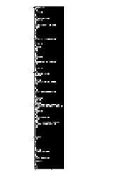Figure 1: Example executable code as an image

In 2010, the authors of [3] used k-NN and feature extraction to achieve 98% accuracy on nearly 9,500 samples of 25 classes of malware. This is one of the earliest works that visualize malware as an image and shows that the concept is viable. The authors note some possible methods of avoiding detection such as inserting redundant bytes. Additionally, we note that this method includes a large amount of preprocessing for the malware images.

In [4], the authors process the images to a standard size and then use a densely-connected neural network to achieve 96.35% accuracy on 3131 files of 24 classes of malware. We note that in this work, excellent results are achieved on such a large number of classes of malware.

More than any other method, the ideas of malware image detection have been combined with the burst of developments with convolutional neural networks (CNNs). CNNs have become the go-to for image classification due to their ability to identify spatial relationships in data [5, 6, 7]. In particular, the Microsoft Malware Classification Challenge has spurred a large interest in using CNNs for malware detection [8]. For instance, the author of [9] used a CNN to acheive 95.24% accuracy on a test set of over 40,000 samples, and then used a residual network to achieve 98.21% accuracy on the same samples. The author also notes that the test set was limited to a certain size of binaries and that future work should expand to any length of binaries. In our own work, which this paper extends, we presented up to 88% accuracy in classifying malware on the same data from the Microsoft Malware Classification Challenge [1] . The largest issue from that work was the large amount of padding used. Instead of reducing or expanding images, we padded all images to be the same length. The upside of this method is that it loses no information, however, there were of course large amounts of padding for tiny images, affecting performance. Like in this work, however, we only used the .text section, proving it possible to only need limited information.

The authors of [10] use a convolutional, distributed network, topped with a recurrent neural network on over 2 million malicious files. The network uses bytes of the full executable without preprocessing and uses and embedding, pointing out the issues with preprocessing. The authors also note difficulties with RNNs due to the length of the sequence, as we also found. The network achieves a maximum of 94% accuracy and 98% AUC. This work is the most similar to ours, however, we expand in a few ways. Most importantly, we are only using the .text section of files, a much smaller subset of the total files. Next, we introduce the concept of breaking the malware image into windows, which would theoretically allow for processing only window at a time, saving large amounts of memory. Next, we apply the ConvLSTM architecture to the data which has not been done before, alleviating RNN issues. We also use global average pooling in one of the final network layers to improve generalization [11]. Finally, we are using a different dataset that is much smaller, but we do achieve better overall performance.

The best performance we could find was by the authors of [12], who combine a CNN and LSTM in ensemble, achieving 99.88% accuracy on 40,000 samples balanced equally between malicious and benign files. Then, when used on only the malicious files, they achieved 99.36% accuracy on 9 classes. Again, the input is the full disassembly of the executables and the input is again preprocessed. Additionally, the authors do not present the method of disassembly for the benign files. We will discuss in the next section some possible flaws with mixing these two types of dataset, of which there may be many.

Executable code as an image has become a hot area of research in recent years. In many of these works the images are preprocessed before classification, which might take a large amount of time or resources in practice depending on the operations, and may be bypassable by reverse-engineering the preprocessing. Additionally, all of the works we have seen use the full executable file for classification. By only using the .text section of an executable, classification can be done at a lower level in the hardware stack, with less memory, less time, and less context of what is running. We will address the issues of using arbitrary-length files by using minimal preprocessing and only using the executable code with a ConvLSTM architecture.

3. Network Input

In our previous work we generated our own data using malware obtained from a Windows installation and live malware found online [1] , number 240 total files split evenly between the two classes. There were a few issues with this dataset, namely, the limited size due to difficulty of acquiring samples and the overly-complex tokenization method. The tokenization of assembly resulted in a larger-than-needed vocabulary size and some preprocessing time which we attempting to limit as much as possible.

As a second test, we used the data from the Microsoft Malware Classification Challenge on Kaggle [8], which contains over 20,000 total malware files from 9 classes of malware. With this data, we are able to directly use the machine code and translate it into decimal per byte, which resembles other works as we have discussed. We will again evaluate performance on this dataset. Of these files, 10,869 had labels and then of those 10,375 were found to have .text sections that we could use, however, we quickly hit memory limits while testing longer files. To solve this, we had to limit to only files that had under 50,000 lines of code, resulting in a total of 8,550 files, of which we used 6,500 training and 2,050 testing files. Because the final goal is classification of malware vs. binary code, however, we have generated an additional dataset consisting of 4,550 benign files from a default Windows installation that were disassembled using IDA pro. Again, due to the 50,000 line cutoff, we were only able to use 3,100 of these files. We then combined the benign data with randomly-chosen malicious files for a second dataset of only malicious vs. benign classification, consisting of 4,000 training and 1,000 testing files.

We will present results on both of these datasets to validate that our own benign files were not biased because of some concerns with the benign data format. While we are comfortable that the datasets are now fair to compare we will show those concerns and how we addressed them. Many benign files were initially identifiable by eye due to some certain characteristics, as in Figure 2:

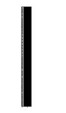Figure 2: First 100 lines of a benign code image

The first problem is that there seems to be a long portion of data bytes at the beginning of many benign files that only includes one or two executable bytes. In the Microsoft dataset, these sections are grouped to have many data bytes per line (up to 18). Next, many lines end in the same color pixel. This is because of how we extract data from the disassembled bytecode – once disassembled from IDA, we simply look at every line to see if it starts with ”.text”, signifying executable code. Then, we extract the hexadecimal bytes from that line until there are no bytes left. Many of these lines end in the byte ”db”, a signal from IDA that represents the variable size (a byte) and not code. For some reason these extra ”db” tokens were never an issue in the Microsoft dataset as there is always some other non-hexadecimal token before them, causing them to be excluded in our extraction. We therefore excluded the ”db” at the end of any line (which is always lowercase if it is not an actual byte in the code but added by IDA, so no innocent bytes were lost). With both of these issues it is possible we are disassembling the data differently than Microsoft did in the Kaggle challenge. Because the exact way that the Microsoft dataset was generated is unknown, we present results on both datasets with the assumption that our benign files are not, but may be, biased.

Unfortunately, malware or benignware can come in all sizes, so the question becomes how to approach classifying arbitrary-length files. Additionally, the files can reach extreme lengths, so a straight LSTM or RNN will experience difficulties in training. We therefore split the files into t windows by grouping every w lines of code. The number of windows forms the new number of timesteps, and the dataset can now be seen as an arbitrary-length sequence of images. An example is shown in Figure 3.

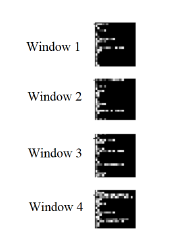Figure 3: Malware Image Windows

Figure 3 shows a malware image split into windows (not to scale).

4. Network Architecture

Forming the malicious bytecode into an arbitrary-length, windowed format allows for input into a variety of network architectures. Before discussing the network architecture for the new input format, we first downsample and perform an embedding on the data. We previously experienced issues with the size of the input being too large to use at once, and even after purposely omitting files over a certain length, the networks would train in an unreasonably long amount of time. Therefore, we utilized pooling to downsample the input data [1] . While this is the only preprocessing we perform, which adds time to making predictions, we still perform downsampling on the data by randomly discarding 9 of every 10 lines. Along with the benefit of faster training and prediction we find that it does not negatively affect performance and actually improves testing performance in some cases, which we will discuss in the results section.

We also previously used embeddings to assist in feature detection, similar to natural language processing [10, 13], as the magnitude of the bytes have no intrinsic meaning. The embedding serves as a look up table where each singular value maps to a higherdimensional space of values with less magnitude.

With the initial layer of an embedding, we now expand on the previously static, convolutional network. A natural pick for classification of these videos would be some kind of recurrent neural network given the time-varying nature and seeming temporal dependency of the problem. In fact, one large question we will pose throughout our work is if the windows are actually temporally dependent, in other words – does the previous window affect how we should see the next? Given the nature of the problem, it seems logical that this would be true, and is the assumption we made for beginning to explore architectures.

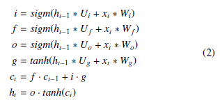
Convolutional LSTMs are a relatively recent form of recurrent neural network that have cropped up in a few field of study that involve both temporally- and spatially-related data [2, 14, 15]. In Keras, this layer of a network is called ConvLSTM2d [16], meaning that it performs 2d convolution inside an LSTM. For comparison, A traditional LSTM uses the following equations:

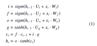Where W_i,f,o,g and U_i,f,o,g are trainable weight vectors, and c_t and h_t are the hidden state and output, respectively. These equations can of course change and are only an example for comparison.

LSTMs can help alleviate ”vanishing gradient” issues when training and therefore allow for training recurrent networks on much longer inputs than a vanilla RNN [17, 18]. We attempted to use a regular LSTM on input mawlware without windows and found that the model would not only take an extraordinarily long time to train, as expected due to the input length, but would not perform well. Even if a decent training accuracy was obtained the results would not translate to testing accuracy.

Recent works, including our own, have shown that classifying malware images responds well to convolution [1] . Therefore, instead of using a LSTM, it is possible to use the Convolutional LSTM (from now on, ConvLSTM). The ConvLSTM consists of nearly the same parts as a regular LSTM except that many dot products are simply switched to being convolution:

Where W_i,f,o,g and U_i,f,o,g are trainable weight vectors, and c_t and h_t are the hidden state and output, respectively.

The ConvLSTM was introduced in 2015 by [2] as a way to capture both spatial and with temporal relations in precipitation forecasting, as opposed to an LSTM, which is only capable of capturing temporal relations. ConvLSTMs have since been used many times to capture spatio-temporal relations in data. In [15], they are used to build on feature extraction in gesture recognition, and in [19], the authors add to the ConvLSTM architecture for traffic accident prediction. More notably, in [20], the authors use a nested ConvLSTM for video classification. Our work can be seen as converting the malware to a video rather than an image, and taking inspiration from these works. In our case, the ConvLSTM captures spatial relations in blocks and functions of code and temporal relations between those blocks.

With the recurrent networks it was found best to use use two hidden recurrent layers, one that returns sequences and a second that does not. When a recurrent network in Keras has the parameter return sequences set to true, the output of the layer is not just the final output but the output of each timestep, the result being a sequence of the same length. Using this parameter is useful as it allows the stacking of recurrent layers and therefore deeper networks.

While our models that use ConvLSTM found success, which we will discuss in the results section, we also found that they took up a large amount of time to train due to the complexity of the hidden state. Many modified RNNs were attempted by removing or adding various gates to the ConvLSTM hidden state until we tested a recurrent network that simply adds the previous hidden state to the current as so:

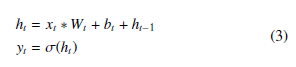Where σ represents the sigmoid function, W_i and b_i are trainable weight vectors, h_t is the hidden state, and y_t is the output at time t.

This network is about as minimal as a recurrent neural network can get and can be compared to a standard recurrent network where the hidden weight vector is set to all 1s. We call this the ”MinConvRNN”. In theory, one layer of this network that does acts the same as if each timestep was independently run through a small neural network and then summed afterwards. Because there are two hidden layers used and each timestep is returned for the first, however, the intermediate timesteps returned by the first hidden layer do not resemble a kind of distributed network.

We can perform backpropogation on the MinConvRNN for training through the widely-known procedure of BackPropogation Through Time (BPTT). We will perform BPTT on the MinConvRNN for completeness, however, gradients are calculated symbolically and automatically in our simulations, so these calculations are not stricly necessary. BPTT consists of unrolling the recurrent neuron into t neurons and repeatedly applying the chain rule. We will start by defining all parameters in Table 1, for any arbitrary objective function J.

Table 1: MinConvRNN Backpropogation Parameters

Variable Name	Purpose
xt	Input at time t
ht	Hidden state at time t
Wt	Weight vector at time t
bt	Bias vector at time t
yt	Output of neuron at time t
σ	Sigmoid Function
δt	∂Jt ∂yt
Jt	Objective function value at time t

The goal of backpropogation is to find the partial derivative of the objective function with respect to a parameter. In this instance, ∂J_{t ∂W}t . Note that Wt for time t is a formality, and W_i = W_j,∀(i, j) ∈ t, and the same for b_i. We begin by defining the base case of t = 1 such that h₀ = 0, making h₁ = x₁ ∗ W₁ + b₁.

Then, we can define the partial derivative of J with respect to W_t using the chain rule:

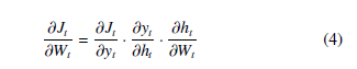We can define δ_t to be ^∂_∂y^Jt^t to simplify notation as the expression will change for a different J. We can then calculate the other terms directly as:

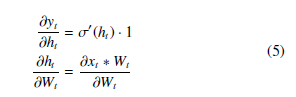We leave ^∂x_∂^t_W^∗Wt ^t alone to simplify the expression, but we note it is computable. It is also known commonly known that σ⁰(x) =, and we will use σ⁰(x) for simplification of expressions as well.

The full partial derivative at time t can then be defined as:

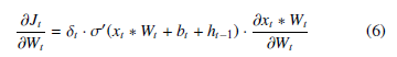Because W_t is the same ∀t as stated earlier, we can compute the partial derivative for W for n timesteps as:

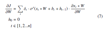For a recurrent neural network where only the output is considered, we could factor out δ_t from the sum. We can also perform a similar process to find the partial derivative for b for n timesteps as

^∂∂b^J = ^Pt δ_t · σ⁰(x_t ∗ W + b_t + h_t−1), with the same conditions.

This partial derivative does not look too dissimilar to that of a basic recurrent neuron. The neuron is indeed recurrent in the sense that it is necessary to calculate h_t−1 in order to calculate h_t, and that the gradient must be propogated starting with the initial output in the same manner. Regardless of these equations, however, the neuron as defined in Eq. 3 does not make intuitive sense. Taking the raw sum after convolution, in theory, might simply lead to an unbounded output in the hidden state that approaches ∞ (or −∞ ) for all elements as the number of timesteps approaches ∞ , leading to all 1s (or 0s) in the output with the sigmoid activation.

As will be shown in the results, we found the MinConvRNN to largely match the performance of the ConvLSTM2d. The success of the MinConvRNN begs the question if a recurrent neural network is necessary, or in other words, if executable code as an image has a temporal dependency when it comes to classification. As will be presented in results, it is even possible to scramble the order of the input lines and achieve decent performance using the same net trained on ordered input lines. It seems unintuitive at first but a simple explanation is simply that a large amount of code is wrapped up in short functions. Depending on how large the window size is made, it is possible that each window encapsulates even multiple functions. Because the order in which functions are defined largely does not matter, there is not a strong temporal dependence between windows. A different explanation may be that even between windows, temporal dependency does not matter, and that the class of a file is largely determined by the types and quantities of commands issued, and not their order. Future work will need to investigate the temporal dependence of the data more closely as it will greatly affect how we classify malware with neural networks.

Regardless of the type, after the recurrent layers, the output has three dimensions. The first two dimensions can be average-pooled to reduce overfitting [11], and then connected with a final denselyconnected layer for the output. The architecture of the network is shown in Figure 4.

5. Performance

We present results on both the Malware Classification Challenge dataset and the Malware vs. Benign dataset as discussed, starting with the Malware Classification Challenge dataset.

Table 2 shows the final results of the ConvLSTM2d and MinConvRNN networks. Both networks were trained until no further performance gains were seen.

Table 2: Results on Microsoft Malware Classification Challenge Dataset

Metric	ConvLSTM	MinConvRNN
Parameter Count	573,634	116,951
Train Accuracy	98.35%	97.28%
Test Accuracy	98.24%	96.39%
Time to Inference	∼63.67ms	∼23.73ms

In Table 2, it can be seen firstly that both networks performed competitively to other works. The MinConvRNN was purposely limited in size to have the same number of convolutional kernels as the ConvLSTM2d network, being 50 kernels of size 4 in the first hidden recurrent layer, and 25 kernels of size 3 in the second hidden recurrent layer. The network was kept the same size to demonstrate the relatively similar performance. While the ConvLSTM2d network did achieve better results, it has nearly 5 times the total number of parameters. Better results are certainly possible through tweaking the network size, activation functions, etc., but we see these networks as a proof-of-concept for future work that does not rely on recurrent networks given the performance of the MinConvRNN. Additionally, we note that the ConvLSTM2d takes nearly twice as long to make a prediction given an input due to the complexity of the hidden state. If we can cut out the recurrent nature of the network, the time to predict would drastically go down.

Table 3 shows Confusion matrix for the ConvLSTM2d network on the testing data, where the row is the actual class and the column is the predicted class. Of note is that one class in the dataset has an extremely low number of samples, class 5. Neither this network nor the MinConvRNN was able to correctly identify and class 5 samples. This might be addressed by using weighted categorical crossentropy, but again, we are presenting these results as a proof-of-concept.

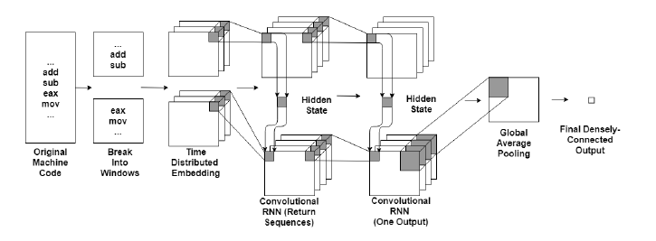Figure 4: RNN for Malware Classification Architecture (for arbitrary hidden state)

Table 4 shows the confusion matrix for the MinConvRNN on the testing dataset, where the rows are the actual class and the columns are the predicted class.

Table 3: Confusion Matrix for ConvLSTM2d Net on Testing Data

Table 4: Confusion Matrix for MinConvRNN on Testing Data

Overall, we see performance for both networks, moreso the ConvLSTM2d, matching other works. The benefit to using these networks is the minimal preprocessing, the small size of the networks, and the minimal amount of input by only using the executable code.

Table 5 shows the results of the networks on the Malicious vs.

Benign dataset.

Results on the Malicious vs. Benign Dataset are on par or better than the previous dataset. Despite reservations with the benign data as previously discussed we believe that the networks show competitive performance in classifying Malicious vs. Benign data to seminal works. The MinConvRNN again shows worse performance than the ConvLSTM, likely due to the smaller number of parameters. Considering that the network is smaller, the relative success of the MinConvRNN calls into question whether using a recurrent network is necessary.

Table 5: Results on Malicious vs. Benign Dataset

Metric	ConvLSTM	MinConvRNN
Parameter Count	573,634	116,951
Train Accuracy	99.78%	99.32%
Test Accuracy	99.50%	99.20%
Test Recall	99.37%	98.12%
Test Precision	99.58%	99.58%
Time to Predict	∼91.16ms	∼35.32ms

6. Future work

There are many topics of future work to expand on. In the big picture, the concept of a non-recurrent network would be interesting to test compared to the recurrent networks. It is possible to take more inspiration from video classification methods in this way. We have observed that a minimal recurrent network achieves decent performance, so with optimization, a purely time-distributed network that is aggregated afterwards may perform well.

With or without recurrent, it would be important to optimize the network, exploring activation function, weighted categorical crossentropy, cross-validation methods, and pruning methods. Performing an architecture optimization search would take much more work, but would improve the performance of the network.

There are also some flaws in our methodology, the largest being the limit of 50,000 line long samples. One possible method of removing this constraint is to reformat the data. The figures of malware code show that each line is padded with 0’s to be the same length – this was done to preserve the ordering of the opcodes in relation to the data. This format, however, may be unnecessary and the code is often treated as one contiguous block in other works. The size of the input would be greatly reduced by removing the padding, which would not only allow for any length input, but also faster and possibly more accurate predictions. Additionally, it would also ensure compatibility with the Microsoft and Benign datasets given the different maximum line lengths.

Finally, finding a way to extend the work to hardware would be great for evaluating the feasibility of the practical implementation of the networks. One possible method of using the malware-detectingnetwork in practice might be to deploy it in a custom chip or FPGA. While the network is likely too large for such acceleration now, with compression techniques, it may be possible to make the network fit. Putting the network in separate, purpose-built hardware would not only free up resources from the main system but also speed up the network considerable.

7. Conclusion

Malware detection will always be a vital part of computer systems. In recent times, classifying malware images made from the executable bytes of a file has become a possible route to take.

This extension of our previous conference paper again proves it is possible to classify malware with nothing other than the .text section of an executable, which contains the actual code that makes up the program. Additionally, we expand on the type of network for detection by creating windows out of the malware image. With this format, minimal preprocessing is required to feed the image into a convolutional, recurrent neural network, achieving competitive performance.

Additionally, we find that using a recurrent neural network may not be entirely necessary. By stripping the ConvLSTM2d of its components and making the MinConvRNN, we have shown that the temporal dependency between windows may not be necessary, opening the doors to new network architectures. Using the MinConvRNN is not the end of the story – it is highly likely that even leaner neural network architectures are possible for malicious assembly.

Conflict of Interest

The authors declare no conflict of interest.

Acknowledgment

The authors would like to thank the University of Cincinnati, Dr. David Kapp at AFRL, WPAFB, OH, and AFRL GRANT No. 1014236 under subaward No. 1919.05.05.91 with TDKC.

1. M. Santacroce, D. Koranek, D. Kapp, A. Ralescu, and R. Jha, “Detecting Malicious Assembly with Deep Learning,” in NAECON 2018 – IEEE National Aerospace and Electronics Conference. IEEE, jul 2018, pp. 82–85. [Online]. Available: https://ieeexplore.ieee.org/document/8556657/
2. X. Shi, Z. Chen, H. Wang, D.-Y. Yeung, W.-K. Wong, W.-C. Woo, and H. Kong Observatory, “Convolutional LSTM Network: A Machine Learning Approach for Precipitation Nowcasting,” Tech. Rep. [Online]. Available: https://arxiv.org/pdf/1506.04214v1.pdf
3. L. Nataraj, S. Karthikeyan, G. Jacob, and B. S. Manjunath, “Malware Images: Visualization and Automatic Classification,” Tech. Rep., 2010. [Online]. Available: https://vision.ece.ucsb.edu/sites/vision.ece.ucsb.edu/files/ publications/nataraj{ }vizsec{ }2011{ }paper.pdf
4. A. Makandar and A. Patrot, “Malware analysis and classification using Artificial Neural Network,” in 2015 International Conference on Trends in Automation, Communications and Computing Technol- ogy (I-TACT-15). IEEE, dec 2015, pp. 1–6. [Online]. Available: http://ieeexplore.ieee.org/document/7492653/
5.  W. Rawat and Z. Wang, “Deep Convolutional Neural Networks for Image Classification: A Comprehensive Review,” Neural Computa- tion, vol. 29, no. 9, pp. 2352–2449, sep 2017. [Online]. Available: http://www.mitpressjournals.org/doi/abs/10.1162/neco{ }a{ }00990
6.  A. Krizhevsky, I. Sutskever, and G. E. Hinton, “ImageNet Classification with Deep Convolutional Neural Networks,” pp. 1097–1105, 2012. [Online]. Available: http://papers.nips.cc/paper/4824-imagenet-classification-with-deep- convolutional-neural-networks
7.  A. Karpathy, G. Toderici, S. Shetty, T. Leung, R. Sukthankar, and L. Fei-Fei, “Large-scale Video Classification with Convolutional Neural Networks,” Tech.Rep. [Online]. Available: http://cs.stanford.edu/people/karpathy/deepvideo
8.  R. Ronen, M. Radu, C. Feuerstein, E. Yom-Tov, M. Ahmadi, and M. . Crowdstrike, “Microsoft Malware Classification Challenge,” 2018. [Online]. Available: http://doi.acm.org/10.1145/2857705.2857713,
9.  A. Singh, “Malware Classification using Image Representation,” Tech. Rep., 2017. [Online]. Available: https://pdfs.semanticscholar.org/5bba/ bd377616bd446a194f432a12e98326f5c637.pdf
10.  E. Raff, J. Barker, J. Sylvester, R. Brandon, B. Catanzaro, and C. Nicholas, “Malware Detection by Eating a Whole EXE,” oct 2017. [Online]. Available: http://arxiv.org/abs/1710.09435
11.  M. Lin, Q. Chen, and S. Yan, “Network In Network,” dec 2013. [Online]. Available: https://arxiv.org/abs/1312.4400
12.  J. Yan, Y. Qi, and Q. Rao, “Detecting Malware with an Ensemble Method Based on Deep Neural Network,” Security and Communica- tion Networks, vol. 2018, pp. 1–16, mar 2018. [Online]. Available: https://www.hindawi.com/journals/scn/2018/7247095/
13.  T. Schnabel, I. Labutov, D. Mimno, and T. Joachims, “Evaluation methods for unsupervised word embeddings,” Tech. Rep., 2015. [Online]. Available: http://www.cs.
14.  J. Donahue, L. A. Hendricks, M. Rohrbach, S. Venugopalan, S. Guadarrama, K. Saenko, and T. Darrell, “Long-Term Recurrent Convolutional Networks for Visual Recognition and Description,” IEEE Transactions on Pattern Analysis and Machine Intelligence, vol. 39, no. 4, pp. 677–691, apr 2017. [Online]. Available: http://ieeexplore.ieee.org/document/7558228/
15.  G. Zhu, L. Zhang, P. Shen, and J. Song, “Multimodal Gesture Recognition Us- ing 3-D Convolution and Convolutional LSTM,” IEEE Access, vol. 5, pp. 4517– 4524, 2017. [Online]. Available: http://ieeexplore.ieee.org/document/7880648/
16.  F. Chollet, “Keras Documentation.” [Online]. Available: https://keras.io/
17.  S. Hochreiter and J. Schmidhuber, “Long Short-Term Memory,” Neural Computation, vol. 9, no. 8, pp. 1735–1780, nov 1997. [Online]. Available: http://www.mitpressjournals.org/doi/10.1162/neco.1997.9.8.1735
18.  K. Greff, R. K. Srivastava, J. Koutnik, B. R. Steunebrink, and J. Schmidhuber, “LSTM: A Search Space Odyssey,” IEEE Transactions on Neural Networks and Learning Systems, vol. 28, no. 10, pp. 2222–2232, oct 2017. [Online]. Available: http://ieeexplore.ieee.org/document/7508408/
19.  Z. Yuan, X. Zhou, and T. Yang, “Hetero-ConvLSTM,” in Proceed- ings of the 24th ACM SIGKDD International Conference on Knowl- edge Discovery & Data Mining – KDD ’18. New York, New York, USA: ACM Press, 2018, pp. 984–992. [Online]. Available: http://dl.acm.org/citation.cfm?doid=3219819.3219922
20.  C. Lu, M. Hirsch, and B. Scho¨ lkopf, “Flexible Spatio- Temporal Networks for Video Prediction,” Tech. Rep. [Online]. Available: http://openaccess.thecvf.com/content{ }cvpr{ 2017/papers/Lu{ }Flexible{ }Spatio-Temporal{ }Networks{ }CVPR{ }2017.pdf

(Click Here)

(Click Here)