1. Introduction

This paper is an extension of work originally presented in 2018 IV International Conference on Information Technologies in Engineering Education (Inforino) [1].

Optimization is a field of mathematics that is widely applied in engineering, e.g. optimal component design and control theory [2, 3, 4]. Traditionally, optimization algorithms are divided into two groups:

• analytic – these are determined algorithms which efficiency and convergence properties are proved; their main disadvantage is relatively poor performance which reduces the scope of applied problems that can be solved by them [5],
• (meta)heuristic – on the contrary, this group of algorithms has problems with the convergence of results: it is not guaranteed that an appropriate solution will be found, but these algorithms are much more computationally efficient and practically verified [6].

The current work consists of several parts:

• Prerequisites – explains reasons which led to the OSOL Extermum development;
• Description of OSOL Extremum – provides information about software structure and technology stack;
• Synthesis of Feedback Control of a Satellite via the OSOL Extremum – describes mathematical task formulation;
• Application Results – demonstrates particular results of application of the developed software;
• Conclusion – summarizes the results and provides information about further research.

2. Prerequisites

In order to understand why the development of a new software was performed it is necessary to describe its background. It will be explained in details in the following subsections.

2.1        Black-Boxing

This is the double-edged sword of software development. On the one hand, it allows one to use given tools without necessity to implement desired algorithm, but on the other – it deprives the opportunity to modify code the way you need it for the exact task. In other words, black-boxing makes all your software tools not as flexible as they can be. Also, you must be totally confident in the quality of the software that you use, because you have no opportunity to check confusing moments.

2.2        Code Reuse

Generally, academic scientists and software developers work differently. Mainly, scientists are more concerned to solve the given problem without any care about reuse of the scripts and software that they have developed. Programmers, conversely, think a bit differently: they use different programming concepts (e.g. object-oriented programming paradigm) in order to maximize the efficiency of written code in future. That gives an opportunity to create reusable tools speeding up further investigations.

2.3        Reproducibility Crisis

Last but not least, reproducibility crisis is general problem for the science. A lot of researches that are described in scientific articles cannot be verified or at least repeated. That happens because of the restrictions on the article size (i.e. there is no enough space to provide step-by-step description or to explain every moment in detail) and displaced informational focus (i.e. scientists are more concerned to present application results not the specification moments).

2.4        Section Summary

Mentioned problems lead to various limits in overall development speed. This coerces scientist to solve tasks that are out of his professional scope. One possible way to weaken effects of described problems is to develop open-source libraries that offer wide capabilities of API (application programming interface) including unified standard for algorithm creation, general testing environment, and huge spectrum of applied tasks.

Available open-source packages (e.g. python’s scikit and scipy packages, R’s specialized packages for optimization) partially solve described problems but mostly provide out-of-box tools. Also none of them fully support interval optimization algorithms and they are hardly connected to external programs. That is why it is important to develop library that can be used as set of building blocks for any desired algorithm.

3. Description of OSOL Extremum

This section provides information about OSOL Extremum presenting its main ideas and features. Source code of the library can be found on GitHub site [7].

3.1        Technology Stack

Software part of the developing library consists of modules that are developed using two program languages: Scala (main logic) and Python (for plotting, scripting, and non-math routines).

Scala belongs to multi-paradigm programming languages which support both object-oriented and functional features [8]. Objectoriented paradigm gives opportunity to develop inheritance hierarchy that simplifies code reuse a lot. Functional paradigm is often treated as more “native“ to mathematicians because its main statements: treating functions as basic objects, data immutability, pure functions, and etc.). Mainly, these statements aimed to provide code stability decreasing places of potential code mistakes. Also. It should be noted that Scala runs on JVM platform, so it is easily maintained and distributed.

Python is a well-known language which is widely used by scientists of different specialization because of its relative simplicity and generous number of various packages (e.g. NumPy, SciPy, Matplotlib, and etc.) [9].

3.2        Library Structure

OSOL Extremum consists of several parts:

• implementation of basic required mathematical operations and objects, e.g. vector operations, function transformations, random number generators, and statistics calculation,
• general template for optimization algorithms that can be extended by other researches to implement desired method,
• block of implemented optimization algorithms,
• block of different tasks (including basic optimization tasks and complicated optimal control synthesis problems).

3.3        Current State and Future Goals

Current version of OSOL Extremum supports the following features:

• definition of basic optimization algorithm in a form of abstract template that supports wide range of running instructions, e.g. termination by max time or iterations and logging instructions,
• bunch of classical and modern optimization algorithms (including Random Search, Simulated Annealing, Cat Swarm Optimization, and Harmony Search) [5, 6],
• tools for the interaction with Simulink models.

In future it is planned to: implement more optimization algorithms, add support of interval optimization algorithms, add support of other modelling systems (e.g. Wolfram Mathematica), add support of other computational cores.

4. Synthesis of Feedback Control of a Satellite via the OSOL Extremum

This section will provide information how OSOL Extremum can be used to solve applied problem in the field of control theory.

4.1        Stage 1: Open-Loop Control Determination

Problem Definition. During the first stage it is required to solve the problem of optimal open-loop control determination.

Let’s consider that the behavior of an object that is described by the following differential equation [10]:

where t ∈ T = [t₀;t₁] is continuous time, T – system operational time, x ∈ Rⁿ – system state vector, u ∈ U ⊂ R^q – control vector, U – set of admissible control values, f (t, x,u) = (f₁ (t, x,u),…, f_n (t, x,u))^T – continuous vector-function. Initial state is given:

terminal state x(t₁) should satisfy the following conditions:

where 0 ≤ l ≤ n, Γ_i (x),i = 1,…,l are continuously differentiable, system of vectors n^∂Γ_∂ⁱ_x⁽1^x),…, ^∂Γ_∂ⁱ_x⁽n^x)o ,i = 1,…,l is linearly independent ∀x ∈ Rⁿ.

The only information which is used to form control is continuous time t. Hence, we consider open-loop control.

Set of admissible processes D(t₀, x₀) is defined as a set of pairs d = (x(·),u(·)) which include trajectory x(·) and admissible control u(·) where ∀t ∈ T : u(t) ∈ U that satisfy equations (1), (2), and (3). On the set of admissible processes we consider cost functional

where f⁰ (t, x,u) and F (x) are given continuous functions.

In order to transform the given problem into the problem without terminal constraints we can use penalty function:

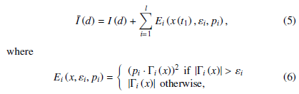are error functions, p_i and ε_i, i = 1,…,l are penalty parameters and maximum allowed errors accordingly.

The task is to find such a pair d^∗ = (x^∗ (·),u^∗ (·)) that

To solve task defined by equation (7) it is suggested to propose parametric form of control and convert initial problem to a problem of parametric optimization. The control, which is obtained by such a procedure, is suboptimal.

Application of Optimization Algorithms. To apply optimization algorithms it is required to parameterize controls in any suitable vector form. Proposed approach was tested using several parameterization schemes:

• polynomial control: (a₀,a₁,a₂,…,a_s)^T ⇒ u(t) = a₀ + a₁ t + a₂ · t² + … + a_s · t^s,
• piecewise linear control: (a₀,a₁,a₂,…,a_s)^T ⇒ u ai + τit+−1−τiτi ai+1, where τi = t0 + i · t1−st0 and τi ≤ t < τi+1.

The value of the cost functional is calculated by the numerical methods using Euler, Euler-Cauchy or Runge-Kutta formulas [11, 12].

To obtain numerical results it is proposed to use two techniques:

• simply generate polynomial control (this technique will be called direct),
• start with determination of controls in polynomial form (with few degrees of freedom) and then use obtained solution as a seed for optimization procedure with piecewise linear controls (this technique will be called sequential).

Transformation, which is used during sequential technique, can be easily done by calculation of values of polynomial control in nodes of uniform grid (demonstrated on Figure 1).

Described techniques differ in this way: direct requires less time to obtain control, sequential requires more time (because of two

parts) but potentially generates more efficient controls (due to bigger number of degrees of freedom).

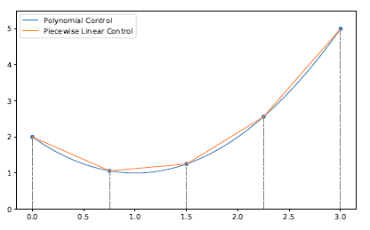Figure 1: Conversion of polynomial control to piecewise linear one

Thus, initial task is transformed to the determination of optimal vector (a₀,a₁,a₂,…,a_s)^T. As the final result of the first stage set of suboptimal controls u˜^∗,k,k = 1,…, K will be found, i.e. u˜^∗,k corresponds to initial state vector x^k (t₀) (K is a number of totally observed initial conditions).

4.2        Stage 2: Controller Construction

Final form of the controller will be found during the final stage in a form of regressor. Current block consists of data preparation part and actually regressor construction.

Data Processing. During current phase initial data will be transformed and modified. There are various data processing procedures [13], e.g.

• This process ensures that only valid data will be used. In our case it is important to include this phase because on previous stage we use metaheuristic optimization algorithms which are not guaranteed to retrieve the best possible solution. Thus, we will eliminate from further consideration those controls which do not provide sufficient accuracy in the means of the final state error defined by equation (8).
• Imputation is widely used in machine learning. Mostly it is present in cases when there is a possibility of data loss. Considered case is determined so there is no need to include it.
• During this phase data, which was previously cleaned, is transformed from raw format (in our case it is set of suboptimal controls) into format that is suitable for machine learning procedures. We will transform data to a table format.
• Normalization is required to standardize obtain data, e.g.

nullify its mean values, normalize standard deviation, etc.

In terms of cleaning it is proposed to use only those controls which correspond to trajectories with relatively small terminal constraints errors, e.g.

where b is a bias value that can be treated as an acceptable level of average cumulative error.

n ^∗,koK it is possible to find Having set of suboptimal controls u˜k=1

corresponding set of trajectories nx˜^∗,koK         from equation (1). This k=1 information is sufficient to build initial dataset that will be considered as a base. Specifically, it is proposed to build dataset in a form of Table 1.

Table 1: Initial dataset template

j(index) t	x1	· · ·	xn	u1	· · ·	uq
1        t j=1	x1 j=1	· · ·	xn j=1	u1 j=1	· · ·	uq j=1
…          …	…	· · ·	…	…	· · ·	…

Such a table can be built for any selected control and then all obtained tables can be concatenated. Thus, we have K different trajectories from each of which we sample in N discrete time moments. Finally, it results into the following bounds for j index: j = 1,…, K · N.

Regressor Construction. Regression is a classical example of socalled supervised learning [14]. In a considered scope of optimal control determination we can treat controls (derived from optimization procedures during the first stage) as an ideal output. Time, and state values can be treated as the input. In other words, desired feedback controller can be treated in this way:

From equation (9) it is obvious how to generate control for previously observed values but it is not clear what to do with new values that will arise in future. That is why machine learning is proposed to be used here – because of its ability to generalize information basing on finite set of observations [15, 14].

In current work it is proposed to build regressor using well known and widely applied Random Forests [16], which are already implemented in Python open-source library Scikit-Learn [17].

4.3        Section Summary

The core component of the described approach is application of optimization algorithms which can be realized via the OSOL Extremum.

Following sections will demonstrate how the proposed approach can be applied to a real control problem.

5. Application Results

5.1        Description of Dynamic Model

To demonstrate the proposed approach the problem of satellite rotational motion dampening is considered [18]. After the conversion to non-dimensional variables system of differential equations, which describes solid body motion relative to centre of mass, will have the following form:

Control vector constraints are represented via intervals ∀t ∈ [0;1]: U = [−500;500] × … × [−500;500].

Cost functional is given by the formula:

         Initial values for      p₀,    q₀,    r₀                   will be taken from sets

{−25, −20,…, −5,0,5,…,20,25} (for direct optimization procedure) and {21,22,23,24,25} (for sequential optimization procedure) which results into 11³ and 5³ possible combinations accordingly.

Terminal constraints are the same for any starting configuration:

Parameters of error functions are also the same for any starting configuration:

Thus, modified functional cost will have the following from:

5.2        Intermediate Results

For All graphics in this and following section horizontal axis is associated with dimensionless time, vertical axis provides information for target variable (also in dimensionless units).

All results in the current section were provided assuming s = 2 for polynomial control and s = 10 for piecewise linear.

Figure 2 demonstrates the obtained results during the optimization stage (for sequential technique).

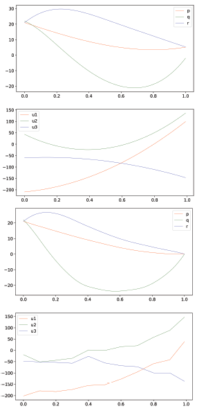Figure 2: Results of sequential optimization procedure for initial conditions p(0) = 21,q(0) = 22,r (0) = 21

From the plot it is clear that during the first stage (generation of polynomial controls) some of them have corresponding trajectories with relatively big errors for terminal state. But it is successfully minimized during the construction of the piecewise polynomial control.

Better visual description of obtained controls can be obtained via bunch graphics demonstrated on Figure 3.

It should be noted that all columns will be scaled (except of the control columns), i.e. transformed to have maximum value equal to 1 and minimum – to 0.

5.3        Final Results

The following section will contain information about obtained regressors. Initial values are chosen in order not to duplicate previously used initial states. Each received trajectory was sampled N = 101 times in moments t_i = 0.01 · i.

Direct technique. Example of application is demonstrated on Figure 4 and Figure 5.

Initial conditions: p₀ = 24,q₀ = 16,r₀ = 16.

       Achieved    terminal   state:       p(t₁)       =       −0.067,q(t₁)       =−0.065,r (t₁) = −0.094.

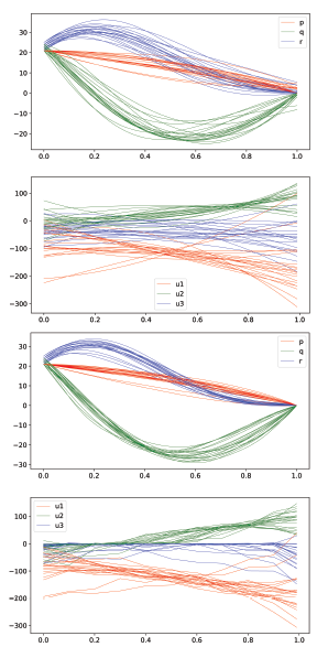Figure 3: Bunches of trajectories and controls (for sequential optimization procedure)

Figure 4: Example 1: trajectories and controls

Initial conditions: p₀ = −9,q₀ = 13,r₀ = −24.

Achieved terminal state: p(t₁) = 0.096,q(t₁) = −0.008,r (t₁) = −0.019.

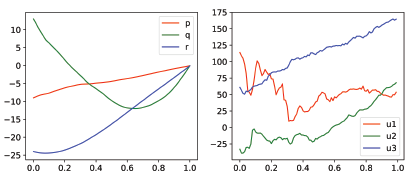Figure 5: Example 2: trajectories and controls

Sequential technique. Example of application is demonstrated on Figure 6 and Figure 7.

Initial conditions: p₀ = 24.7,q₀ = 23.3,r₀ = 21.1.

Achieved terminal state: p(t₁) = 0.101,q(t₁) = −0.063,r (t₁) = −0.002.

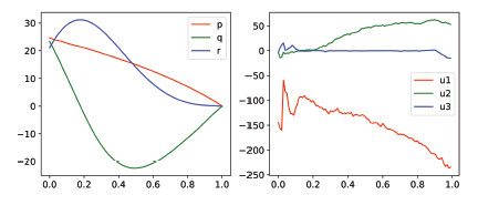Figure 6: Example 3: trajectories and controls

Initial conditions: p₀ = 21.1,q₀ = 21.2,r₀ = 21.3.

Achieved terminal state: p(t₁) = 0.09,q(t₁) = −0.067,r (t₁) =0.058.

Figure 7: Example 4: trajectories and controls

From observed graphics it is evident that the proposed approach has a great potential to solve the problem of feedback control synthesis. Disadvantage of the proposed approach is that obtained controls are not smooth functions. Such particularity is treated as a disadvantage because it complicates the hardware implementation of the generated control and lowers durability of control mechanism due to the necessity of high-amplitude control adjustments.

6. Conclusion

Main results of the current work are the following:

• efficiency of the developed OSOL Extremum software complex was proved based on obtained solutions for tasks of open-loop control determination,
• proposed approach was tested on an applied task of satellite rotational motion dampening.

Further research is planned to be conducted in several different directions:

• find the way to make controls, that are generated by regressors, have smoother form,
• determine losses in efficiency in the terms of cost functional compared to other computational approaches (including analytic ones),
• find the way how to conduct proper comparative analysis and provide detailed comparison report with the existing software complexes in the terms of accuracy, computational efficiency, and algorithm coverage.

1. Panteleev A.V., Panovskiy V. “2018 IV International Conference on Information Technologies in Engineering Education (Inforino)“ in 2018 IV
   International Conference on Information Technolo- gies in Engineering Education (Inforino), Moscow, Russia, 2018. https://doi.org/10.1109 581745
2.  Panteleev A.V., Panovskiy V. “2018 IV International Conference on Information Technologies in Engineering Education (Inforino)“ in 2018 IV International Conference on Information Technolo- gies in Engineering Education (Inforino), Moscow, Russia, 2018. https://doi.org/10.1109/INFORINO.2018.8581745
3. Panteleev A.V., Letova T.A., Pomazueva E.A. “Parametric Design of Optimal in Average Fractional-Order PID Controller in Flight Control Problem“. Automation and Remote Control, 79(1): 153 – 166, 2018. https://doi.org/10.1134/S0005117918010137
4.  Kuo Y.-L., Wu T.-L. “Open-loop and closed-loop attitude dynam- ics and controls of miniature spacecraft using pseudowheels” Com- puters and Mathematics with Applications, 64: 1282 – 1290, 2012. https://doi.org/10.1016/j.camwa.2012.03.072
5.  Panteleev A.V., Panovskiy V.N., Korotkova T.I. “Interval explosion search algorithm and its application to hypersonic aircraft modelling and motion optimization problems“. Bulletin of the South Ural State University, Series: Mathematical Modelling, Programming and Computer Software, 9: 55 – 67, 2016. https://doi.org/10.14529/mmp160305
6.  Bazaraa M.S., Sherali H.D., Shetty C.M. Nonlinear programming. Theory and algorithms, New York, John Wiley & Sons, 2006.
7.  Gendreau M., and Potvin J.-S. Handbook of Metaheuristics, New York, Springer, 2010.
8.  GitHub: Open-Source Optimization Library – Extremum. https://github.com/wol4aravio/OSOL.Extremum
9.  Odersky M., Spoon L., Venners B. Programming in Scala, Walnut Creek, Artima Press, 2016.
10.  Lutz M. Learning Python, Sebastopol, O’Reilly Media, 2013.
11.  Panteleev A., Bortakovskiy A. Control Theory in Examples and Problems (Teorija upravlenija v primerah i zadachah), Moscow, Viskaya Shkola, 2003.
12.  Panteleev A., Metlitskaya D. “An application of genetic algorithms with bi- nary and real coding for approximate synthesis of suboptimal control in de- terministic systems“, Autom. Remote Control, 72:11, 2328 – 2338, 2011. https://doi.org/10.1134/S0005117911110075
13.  Panteleev A., Metlitskaya D. “Using the method of artificial im- mune systems to seek the suboptimal program control of determin- istic systems“, Autom. Remote Control, 75:11, 1922 – 1935, 2014. https://doi.org/10.1134/S0005117914110034
14.  VanderPlas J. Python Data Science Handbook, Sebastopol, CA: O’Reilly, 2017.
15.  Herbrich R. Graepel T. Machine Learning: An Algorithmic Perspective, Boca Goodfellow I., Bengio Y., Courville A. Deep Learning, Cambridge, MA, MIT Press, 2016.
16.  Breiman L. “Random Forests“. Machine Learning, 45(1): 5 – 32, 2001. https://doi.org/10.1023/A:1010933404324
17.  Hackeling G. Mastering Machine Learning with scikit-learn, Birmingham, Packt Publishing, 2014.
18.  Krylov I. “Numerical solution of the problem of the optimal stabilization of an artificial satellite“. USSR Computational Mathematics and Mathematical Physics, 8(1): 284 – 291, 1968. http://dx.doi.org/10.1016/0041-5553(68)90021-9

(Click Here)

(Click Here)