1. Introduction

Feature objection extraction [1, 2] is an evidence accrual technique that can be applied to classification problems. An undirected tree [3] with various levels of information is used to connect evidence nodes. Each node has a level of evidence and an associated level of uncertainty similar to a state in a Kalman filter. Within the tree, nodes represent levels of evidence of what might be elementary information or a complex combination of information. This paper extends work originally presented in the 2018 Conference on Innovations in Intelligent Systems and Applications [1]. In theory, every node can be measured directly or indirectly. Unlike typical evidence accrual methods [4-6], the states are not probabilistic. When evidence points to more than one solution, multiple competing solutions can each have levels of evidence. Evidence can affect nodes at the same level, with the same evidence potentially increasing one or more than one node in levels of evidence, while others may have their levels decreased, and still other nodes at the same level may not be affected at all.

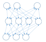Figure 1: Feature-object extraction structure with various interconnections in a multi-level tree

      Feature objection extraction (FOX) propagates information within the tree using a variety of function or function-approximation relationships. The measured information is injected using a fuzzy Kalman filter [1, 7]. As will be described in detail, the FOX evidence accrual system decomposes high-level concepts into simpler concepts until it reaches root nodes which are comprised elementary information. Figure 1 describes a basic FOX tree with different connections and a variety of level of elementary information.

      FOX is incorporated into a tracking system to detect a target’s maneuver and can use the computed values of the track to produce a measure of evidence that maneuver is occurring. Maneuver detection is important because, if the target dynamics are not modeled correctly for a maneuver, the tracking system can have an offset or a time-lag in its estimation of the target position and velocity. In Figure 2, an example of a maneuvering target trajectory is shown, alongside the target track from a Kalman-filter based tracking system, a more typical approach. The figure shows a track lagging the true target trajectory as the target proceeds through the maneuver. This comparative result illustrates the deleterious effects that can result when a maneuver occurs. Tracking problems also become more prevalent when the measurement lies in the unobservable space of the track kinematics, as seen in [8]. For example, if an angle-only tracker is used, the filter can become numerically unsound and require a reinitialization. In the tracking problem, losing a target or creating large target kinematic-errors can be life-or-death issue. If a maneuver can be detected, the tracking algorithm can be modified to improve performance and avoid catastrophic failures.

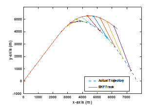Figure 2: Ballistic target and standard tracker result in lagging of track through maneuver

The Kalman filter, and its numerous variants, such as the extended Kalman filter (EKF) [9] and the unscented Kalman filter [10], have long provided the predominant core approaches for kinematic target-tracking systems [11]. To reduce the deleterious effects that maneuvers have on a tracking system, compensation approaches have been developed. The most widely used technique is the interacting multiple model (IMM) and its variants [12]. The IMM incorporates various maneuver models. The IMM system creates weighted combinations of models by comparing the residuals of each measurement to each model’s prediction. The residual scores are used to interpolate between the models and create a weight for the state of each motion model to create a more accurate state estimate of the target position and velocity. Other techniques include adaptive Kalman filters such as a neural extended Kalman Filter (NEKF) [13] that also employ the Kalman filter residuals to adapt their maneuver parameters to more closely model that of the actual target dynamics.

All of these approaches rely on the residual measures to detect and make the adjustments. While the residual is an effective measure, variations in uncertainty can mask the maneuver until the residual value becomes significantly large. Fortunately, there exist other metrics as part of the Kalman filter that can detect a maneuver. Besides the residual, the behaviors of the Kalman gain can also indicate that the target is in a maneuver.

FOX can be employed to combine the disparate information and the associated uncertainty, providing for an effort at detection based upon more than one type of measure. In the problem demonstrated in this work, there is an injection of Kalman gain data provided by the aforementioned fuzzy Kalman filter, augmenting the residual measures, and the evidence is propagated using fuzzy, linear, and nonlinear relationships.

 Four further sections provide an overview of the development of this approach and analyze its capability. Section 2 overviews the EKF, the most prominent variant of the Kalman filter used in tracking that provides the Kalman gains. Section 3 describes the Kalman gain behaviors that can provide information measures to indicate a target maneuver. Section 4 describes the FOX evidence accrual maneuver detection technique. In Section 5, examples of maneuvering targets are described and are used to exemplify the capabilities of FOX as a maneuver detection technique.

2. Target Tracking with the Extended Kalman Filter

      For kinematic target tracking, the discrete-time dynamics of the are defined in (1).

The subscript k indicates discrete time, and x is the standard state-vector representation of the target behavior represents position and velocity. In (2), the state vector represents three dimensions

      The target dynamics F are often described with the straight-line motion model

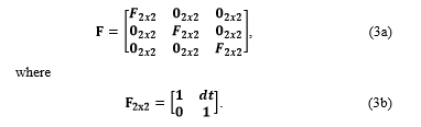The term dt is the time difference between the last sensor report on the target and the latest sensor report.

      While the dynamics are linear, the measurements provided by sensors are often nonlinear. Using active sensors, such as radar, a complete measurement space for the three-dimensional target-track would be a report h(x) of range, bearing, and elevation, shown in (4)

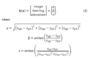and the subscript tgt denotes target component and the subscript plt denotes the platform.

      Since these measurements are generated relative to the sensor platform, when they are reported to the tracking algorithm, they may be transformed to a universal coordinate system, such as earth-centered-earth-fixed (ECEF), be relative to the tracking system, or be relative to a localized flat earth [14]. To maintain the accuracy of the measurement, though, it is kept in a nonlinear-coordinate frame rather than being mapped into the track-coordinate frame which would linearize the tracking system.  This is one reason the extended Kalman filter (EKF) is the most prevalent tracking algorithm [11].

      These measurements are the driving inputs for the tracking algorithm. The EKF uses its estimate of the measurement and the residual between the estimated and reported measurements to correct its state-estimate of the target kinematics. The process of EKF to accomplish this is defined in (5a-e)

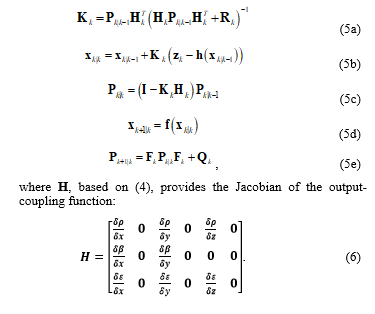
The function f is the modeled target dynamics, and the matrix F in (5d-e) is the associated Jacobian. As stated previously, the target dynamics are usually defined as (3a). The subscript indicates discrete time, with k|k is the estimate at the time k given all the information up to that time and k+1|k is the estimate for time k+1, given all the information up through time k.

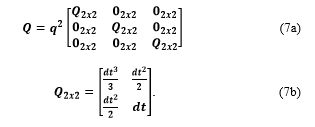
The process noise, Q, indicates the accuracy of the system dynamics, and is usually modeled as integrated white noise [15]:

      As the process noise is increased, the dynamic model, F, in (5d‑e) is weighted less. The measurement becomes more dominant in the processing, allowing more of the measurement noise to be passed thought the filter to the track solution. As the process noise is decreased, in contrast, the reaction of the tracking algorithm becomes less responsive to the measurement and more smoothing occurs.

While not explicit in the (5a) and often overlooked, the EKF’s Kalman gain is affected by the process noise, the error covariance P, and the state estimate x. The state estimate is injected into the Kalman gain though the output-coupling Jacobian H. The gain is also affected by the measurement noise R. The measurement noise relates to the quality of the sensor. A standard radar will have its angle accuracies based on its beamwidth, for example while the range accuracy will be based on the resolution of the pulse signal. The accuracy indicates that the target can be anywhere within the beam and so-called range bin, as with airborne radar.

Since a Kalman filter is used, the accuracy is represented as a Gaussian distribution. (If the accuracy is not Gaussian, techniques such as Gaussian sums could be used to represent the measurement accuracy [16], but that is beyond the needs of these developments.) In Kalman filtering, the ratio of Q to R represents the relative belief of the target-motion model versus that of the sensor reports. If Q is smaller relative to R, the measurements will have a reduced of effect on the target track and the results from measurements over time will be smoothed, with the effects of noise less pronounced. If this ratio is reversed, the measures will dominate the track behavior, with the effects of individual measurements more pronounced in the target track. It is of note that, since the EKF is a measurement driven method, measurements will always ultimately have some effect on the target track. When the measurements noise is smaller, the measurement effects will have a faster impact on the track as sensors are viewed as more accurate.

3. Kalman Gain Monitoring

The extended Kalman filter (EKF) behaves differently than the Kalman filter for linear time-invariant systems. While the Kalman filter for such systems is predictable in nature, the EKF will vary over time. The variations in the error covariance P are affected by the nonlinear behavior of the system and the local estimate in both the update equation of (5c) and the prediction equation of (5e).

The behavior of the Kalman gain within the EKF, the vector K, often precedes the noticeable changes of the error covariance. This arises as the Kalman gain is affected both by the nonlinearities directly in (5a) and by the variations in the error covariance matrix. As the gains change over time, the filter can inherently detect changes in the actual system that vary from the estimation model. In [1], for a target tracking application of the extended Kalman filter, the Kalman gains demonstrated that over time there existed features in their behaviors that coincided with target maneuvers. The analysis of [1] looked at the individual gains, tracking both position and velocity of the targets in two-dimensional space using a range and bearing measurement. The resulting behaviors of the eight element Kalman-gain vector were used as features to identify when various maneuvers, including turns and simple linear accelerations, occurred. Another example is provided here.

The details of the scenario are shown in Figure 3. The target simulates the behavior of a submarine as it is being tracked by another vessel. The submarine maintains a straight-line trajectory with a constant speed. The trailing vessel also maintains a constant speed and course. After some time, the target maneuvers. This represents a concept in a submarine-tracking problem where, being tracked, the target maneuvers to clear baffles to “see” the trailing ship and possibly cause a break-in-track of the enemy’s tracking system. The platform ship then maneuvers, followed quickly by the submarine maneuvering again. These successive maneuvers can result in the filter becoming numerically unsound.

Figure 4 shows the behavior of the four Kalman gains related to the range over this whole scenario and is marked where the target and the sensor platform perform maneuvers. The Kalman gains show different behaviors, including a sharp transient, a significant change in the slope of the gain, and a zero-crossing.

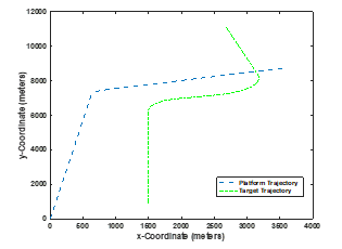Figure 3: A manuevering target being tracked by a maneuvering sensor platform

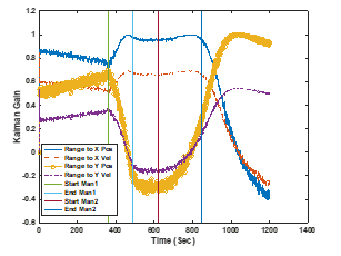Figure 4: The behavior of the range-related Kalman gains over the course of the scenario with the target maneuvers marked

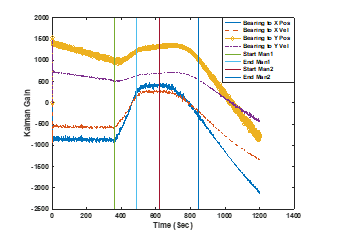Figure 5: The behavior of the bearing-related Kalman gains over the course of the scenario with the target maneuvers marked

The other four gains, which relate to the bearing measurements, are shown in Figure 5, and are larger in magnitude, but similar in relative behavior. Other test cases [1, 17], have also shown the gains to high frequency behaviors during maneuvers.

From these various test cases, the features of interest to detect a target maneuver have been determined to include monitoring the frequency behavior, the zero-crossings, the transient behavior, the slope performance, and the ownship (platform) maneuvers.  It has also been determined that only a subset of the Kalman gains are necessary to observe. These include the gains related to the position states and range measurements K₁₁ and K₃₁ and all of the gains related to the bearing measurements K_i2, where those required vary by feature

4. Evidence Accrual Using Feature Object Extraction

      Many evidence accrual methods have been developed to combine information which, in this case, provide a level of evidence that a maneuver is occurring or has ceased to be. The primary evidence accrual techniques are the Dempster-Shafer method [5] and the Bayesian taxonomy approach [4], also referred to as the Pearl Tree. While these techniques have been utilized for decades, they have drawbacks, including that both represent the information as probabilities that update following Bayes rule. Also, uncertainty in the information that is the basis of the probabilities is not modeled easily, even with Dempster-Shafer.

      FOX provides for distinct levels of evidence, such as of maneuver and for a non-maneuver separately. Since the measures of evidence are generated independently, the scores, unlike probabilities, are not related and an increasing evidence for one decision (i.e., a maneuver) need not decrease the other decision (i.e., no maneuver). Evidence can prove one or multiple decisions thus changing all or some of the decision.

      FOX is also designed to provide a quality score with each level of evidence. The quality score is similar to a Kalman filter error covariance in that a high score indicates uncertainty while a low score indicates a high degree of certainty about the evidence score. The corroboration of evidence gathered from various behaviors can improve the certainty that an event occurred. Conversely, with multiple sources of evidence, maneuver events can be detected with one gain behavior being triggered while the others have not met the threshold.

For the maneuver detection problem, each of the elements of the Kalman gains’ behaviors from the target tracking system can be used individually to indicate when a target maneuver is being initiated.

      The FOX technique is designed to decompose a complex classification problem into a series of smaller and simpler problems. For the maneuver detection problem, a unidirectional tree is employed, as shown in Figure 6, illustrating use of FOX to accrue evidence based upon multiple behaviors of the Kalman gains. For maneuver detection, the top level is Detected Maneuver. The degree of evidence for this evidence node is limited to a range between 0 and 1. A corresponding tree for determining a level evidence for no maneuver occurring would be similar in concept with different linkages. The next level of this tree is comprised the individual-event detections of the tracking-system’s Kalman gain vector: Zero Crossing, Gain Frequency, and Slope Variation. These three components are combined to create the Detected Maneuver scores. As the evidence levels in these states increase from 0 to 1, the overall detection-levels vary based not only on the lower-level scores but the quality level as well. Poor quality scores are weighted less than higher quality scores.

In Figure 6, the shaded states indicate elementary-evidence input nodes. These represent the elemental measurements such as the measured frequencies or number of zero crossings. The unshaded nodes are referred to as states of interest. These are states of combined information.

Another important aspect of the approach is that, unlike the states of Markov chain [6], these states need not be disjoint nor do the states need be a complete representation of all the states of the system.

While the Kalman gain elements of the target tracking system provide evidence to the FOX evidence accrual system which employs a Kalman filter itself. To clarify, the Kalman filter of the FOX system in this case, actually a fuzzy Kalman filter, is different than that of the tracking system that is a source of evidence.

The level of evidence for a state of interest can be generated in two ways. The first is through direct observation, which implies a direct measurement is available, as shown with the shaded nodes. The evidence is then processed through a substate, depicted with a clear node. The tree of Figure 6 shows some substates have multiple injection nodes flowing into them. The FOX Kalman filter that injects the evidence into the tree nodes is a fuzzy Kalman filter (FKF). The FKF takes the multiple inputs and creates a single-output fuzzy measure. Substates that do not have direct evidence injection are generated using systems theory. The substates connect to state of interest through links that represent the functional relationship.

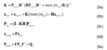
The FKF of the FOX system is based upon a development of Watkins [7] and modified in [2]. This approach was selected to allow a wide variety of measurement types and uncertainty models to be used with ease. The FKF implementation is a straightforward variant of the standard Kalman filter with a modification in the update equations. The FKF is defined in (8) with five equations, (8a) to (8e). Comparing the sets of equations, (5) and (8), two of these, the Kalman gain equation of (5a) and (8a), and the state update equation of (5b) and (8b), are the ones where counterparts differ. The fuzzy measures are incorporated by using the first moment, indicated as mom₁, of the consequent fuzzy membership function, referred to as , or the membership adjunct.

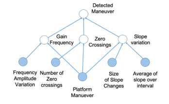Figure 6: The proposed evidence accrual tree decomposition for Kalman gain maneuver detection approach of FOX

The use of fuzzy logic provides for simplified linguistic based conversion from the measurement coordinate systems to the evidence space, which has been defined as a value between 0 and 1. If the measurement and uncertainty values are crisp, the FKF devolves into the standard Kalman filter.

The nature of the measurement data determines whether the fuzzy measure or a crisp measure is used. A true measure such as the number of zero crossings or a known even as the knowledge of a platform maneuver would be a crisp value that would map into crisp groupings. The mapping of data into groupings, such as a determination based upon the frequency behavior or degree of slope change, would be fuzzy.

Once elementary evidence is injected into the tree, it can propagate another FKF process or through the use system theory process as follows. A state of interest and its direct-substates are represented in vector form as

The state of interest or of the node value is the first element of the state vector.

Using first-order observer decomposition [18], the evidence dynamics are given as

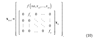The state of interest is comprised of its substates and the previous value of the state of interest. The observer concept provides a forgetting factor. This forgetting factor and the observer updating equation are used to incorporate the quality factor of each sub-state. In (10), the uncertainty can be incorporated as a simple scaling in the state values or in the state-of-interest function, . The associated error covariance or uncertainty equation is propagated by (11).

 This decomposition of the problem into the individual substates reduces the complex model of the interactions of information into simplified operations. The decomposition also simplifies the incorporation of the uncertainty into the state vector.

4.1.  Maneuver Detection Fuzzy Membership Functions

To generate the injection evidence, the following antecedent and consequent functions along with their associated inference engines were considered:

4.1.1. Frequency Amplitude Variation

          When a maneuver occurs, some Kalman gain elements experience high frequency changes in amplitude. The high frequency behavior indicates that a maneuver could be occurring. As seen in [17], the high frequencies indicate potential issues with the Kalman filter that are a result of sharp maneuvers. The frequencies are mapped into a score using two input antecedent functions: Max_frequency_value and Ratio_of_high_frequency_to_low_frequency_power.

          Figure 7 provides a four-element antecedent function that breaks the fast Fourier transform (FFT) spectrum of a time slice of the Kalman gain maps into the four trapezoidal-based functions. Figure 8 shows the five-element triangular antecedent membership functions that represents the ratio of the power of the highest-tenth of the spectrum to the lowest tenth of the spectrum. Table 1 provides the inference engine of the two sets of membership functions. These map to the consequence functions shown in Figure 9. These are defuzzified using the FKF.

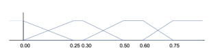Figure 7: Kalman Gain Frequency amplitude variation FFT time slice antecedent function

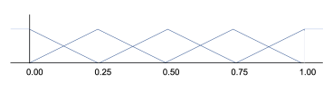Figure 8: Kalman Gain Frequency amplitude power ratio membership function

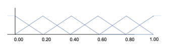Figure 9: Kalman Gain Frequency Consquence Function

Table 1: Kalman Gain Frequency Inference Engine

	Frequency Maximum Membership Function
Frequency Power Ratio Membership Function	1	2	3	4
1	1	2	3	4
2	1	2	4	4
3	2	3	4	5
4	2	4	5	5
5	3	4	5	5

4.1.2. Number of Zero Crossings

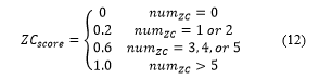
The number of zero crossings is a crisp value. The number of zero crossings  is mapped into a score :

4.1.3. Slope Changes

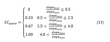
        The size of the slope changes in a given time interval is measured. The value is an absolute value of the difference between the initial slope and the ending slope compared to the maximum and minimum values. This crisp value is mapped similarly to the number of zero crossings but, are mapped evenly across four regions are mapped into the scores:

Unlike the other injection evidence mentioned here, the uncertainty is also fuzzy. The size in the slope changes creates the next score. Figures 10 depicts a five-element trapezoidal function that map the change in slopes. Table 2 provides the inference engine that maps into the consequence function represented by five triangular functions as seen in Figure 11. Again, the defuzzification is performed by the FKF.

Table 2: Kalman Gain Slope Inference Engine

Slope Average Membership Function	0.0	0.33	0.67	1.0
1	1	1	2	3
2	1	2	3	3
3	3	3	4	4
4	5	5	5	5
5	5	5	5	5

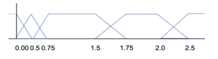Figure 10: Changes in Kalman Gain Slope Membership Function

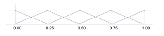Figure 11: Changes in Kalman Gain Slope Consquence Function

  Now that the direct evidence has been defined, the higher level nodes, depicted in Figure 4, can also be defined. The function relating the three sets of substate evidence to the Detected Maneuver state is defined with the limited linear combination in (14).

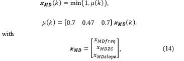where (k) is the estimated level of evidence at time k for detection of a maneuver state. The states that comprise  are , the frequency behavior of the Kalman gain used to detect a maneuver, , which is the incidence of zero-crossings for a Kalman gain value, and , which is the change in slope of the Kalman gain value that indicates a manuever. For , the score was not directly weighted by the measurement uncertainty and is solely based on the current values of the components.

The subnode x_MDZC is defined at time k as

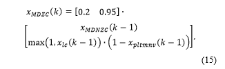where  is either 1 or 0, with a 1 indicating the platform is, and a 0 indicating that it is not, in a maneuver at time k.  is defined based upon whether the measurement is range-bearing in (16) or bearing only in (17), using elements of the Kalman gain. For range-bearing,

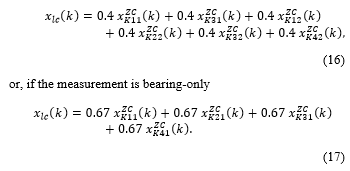
Here, the subscript Kij indicates the ith, jth element of the Kalman gain and  indicates the Kalman gain number of zero-crossings upto time k.

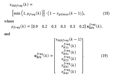
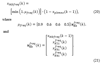
The subnode x_MDfreq is defined in (18) and (19) for the range-bearing measurement and in (20) and (21) for the bearing measurements.

For the range-bearing subnode ,

For the bearing-only measurement, the subnode x_MDfreq is defined similarly, but with different Kalman gains, as

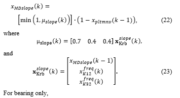
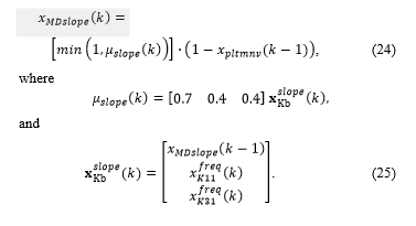
Finally, the subnode x_MDslope is defined in (22) and (23) for range-bearing measurements and in (24) and (25) for bearing-only measurements. For range-bearing,

5. Scenario, Example, and Analysis

      In each of two examples, an EKF target tracking system is employed and the FOX system as previously described is applied. The scenario used to demonstrate the effectiveness of FOX technique as applied to the maneuver detection problem was summarized in Section 2 and is illustrated in Figure 3. The simulator was developed in MATLAB by the authors. The scenario lasts 1200 seconds. A platform is heading 5 degrees west of north for 480 seconds at 15 kts. Then, the platform changes heading and speed over 60 seconds to 65 degrees west of north and to 9 kts. The platform remains at this heading and speed for the rest of the scenario. The target heads due north for 360 seconds at 15 kts. Then the target changes course and speed over 130 seconds. The course is changed to 70 degrees west of north, and the speed is slowed to 10 kts.  At 620 seconds into the scenario, the heading and speed is changed again. This time the acceleration of the target is changed over 224 seconds. The speed is changed to 15 kts while the heading is changed to 10 degrees east of north.

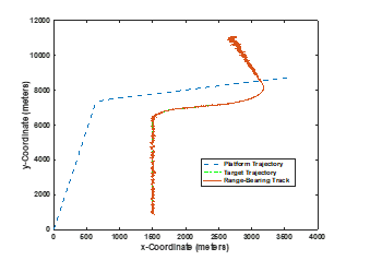Figure 12: The test scenario with the tracked target using range and bearing meaasurements.

The platform sensor in the first example is a range-bearing sensor with a reporting time of 1 second. The range accuracy is 0.01 m while the bearing accuracy is 0.0003 radians. In the second example, the range sensor is turned off, while the bearing sensor has the same sample time and accuracy in the first example.

5.1.   Example 1

The target track of the scenario when using the range-bearing measurement is shown in Figure 12. The associated Kalman filter gains associated to the range measurements are seen in Figure 4 and the gains associated to the bearing measurements were provided in Figure 5. The gains are windowed over a 20 second segment. The window continually slides until the end of the scenario.  Figure 13 shows the resulting maneuver detection score.

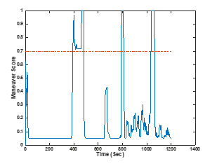Figure 13: FOX maneuver-detection system results for the range-bearing example

The maneuver detection results indicate that the FOX maneuver detection does detect the target maneuvers when the measurements driving the tracking system contain both a range and a bearing. Using a detection threshold of 0.7, the first target maneuver is detected 31 seconds after it begins (near 400 seconds into scenario) and FOX continues to detect it until the platform begins its maneuver. The second maneuver is detected 170 seconds into its 224 second increase-in-speed and turn. When the target switches from east to west in absolute bearing, the event is detected as a maneuver for 30 seconds. The sharper maneuver (the first maneuver) is detected earlier and for a longer percentage of time of the maneuver. The maneuver has a significant effect on the range and bearing change and impacts the Kalman gain relatively more than a measurement that has little relative impact as with the second maneuver.

In the second maneuver, the effect on the Kalman gain vector values is smaller; the change in bearing and range is smaller at first, and then builds. This compares similarly to the results in [1, 17] in that the closer a target is to the platform and the sharper the maneuvers, the greater the Kalman gain behavior. When the target moves from east to west of the platform, the bearing changes from positive to negative. While the tracker handles the transition smoothly, the sign-changes affect the Jacobian of the measurement-coupling function H, as in Eq. (5a). This would be the same if the platform were to maneuver. The results indicate that using the Kalman gains are able to provide indication of maneuvers. The underlying scores indicate that slope behavior is important in target turns. The frequency behavior complements the zero-crossing in the last two detections.

5.2.  Example 2

Figure 14 shows the target track overlaid the truth track for the scenario. The target track is, as expected, terribly inaccurate as bearing-only measurement makes the target location and velocity partially unobservable [19]. The target also maneuvers, and this exacerbates the issue [20]. The associated Kalman gains are shown in Figure 15.  The Kalman gains are similar to the bearing gains of range-bearing measurement of Example 1. The gains are windowed over a 20 second segment. The window continually slides until the end of the scenario.  Figure 16 shows the maneuver detection score.

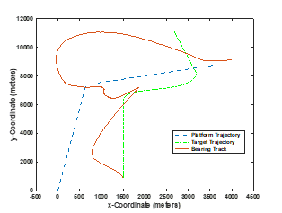Figure 14. The test scenario with the tracked target using bearing-only measurements where the target position and velocity become unobservable

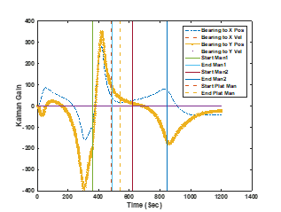Figure 15: The bearing-only related Kalman gains as mapped over the entire scenario with target and platform maneuvers indicated

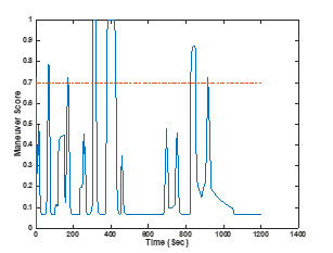Figure 16: FOX maneuver-detection system results for the bearing-only tracker

The maneuver detection algorithm shows six detections of maneuvers. As discussed in [8], the estimations from a bearings-only track have significant observability issues. The fact that the target is moving originally parallel to the sensor platform results in the range information not being observable. This often collapses the range uncertainty covariance. Three times the target track is detected as a maneuver. In watching the tracker behavior, the Kalman gain is actually providing indications of the failure of the tracking system. When the target maneuvers, the algorithm detects this behavior as the EKF becomes more inaccurate. The platform maneuver provides a pseudo cross-fix which temporarily corrects the track but does not provide enough information to stabilize the filter. The second maneuver is detected later than the maneuver when the range-bearing tracking. For this unobservable measurement type, the FOX algorithm will detect issues with the tracker performance besides maneuvers.

5.3.  Summary of Results

The two test scenarios indicate that the FOX maneuver-detection algorithm was able to provide triggers when the target is in or concluding a maneuver. The algorithm also detects other events, particularly the failure of the EKF. This would indicate that at times a reset in the tracker could be useful. It also indicates that behaviors, such as the change from east-to-west of the target, needs to be incorporated into the algorithm similar to the platform maneuver.

6. Conclusions

In this paper, the FOX evidence accrual technique was applied to the problem of detecting target maneuvers using measures from the Kalman gain behaviors from an EKF tracking routine. The algorithm was demonstrated to a variety of events most notably, when the trackign system begins to numerically collapse. Kalman gains of an EKF are important element in detecting tracking failures or changes. The results indicate that other highest-level nodes,i.e., target cross-overs and Kalman collapse, should be incorporated into the FOX system. Maneuver detection can be exploited to work with EKF tracking systems. Incorporation of the method into an interacting multiple-model (IMM) tracking system is planned to advance the applicability of the technique.

Conflict of Interest

The authors declare no conflict of interest.

1.  S.C. Stubberud, K.A. Kramer, and A.R. Stubberud, “Fuzzy-Based Evidence Accrual for Target Maneuver Detection,” in Proc. of Innovations in Intelligent Systems and Aplications, INISTA ’18. 2018, pp. 1-7. https://doi.org/10.1109/INISTA.2018.8466310
2.  S. Stubberud and R. Pudwill, in “Feature object extraction – a fuzzy logic approach for evidence accrual in the Level 1 Fusion classification problem,” in Computational Intelligence for Measurement Systems and Applications, 2003. CIMSA ’03. 2003 IEEE International Symposium on, 2003, pp. 181-185. https://doi.org/10.1109/CIMSA.2003.1227224
3.  R. Sedgewick and K. Wayne, Algorithms, 4th Edition, Addison-Wesley, 2011.
4.  J. Pearl, Causality: Models, Reasoning and Inference, 2nd Edition ed.: Cambridge University Press, 2009.
5.  A. P. Dempster, “Upper and lower probabilities induced by a multivalued mapping,” Annals of Mathematical Statistics, vol. 38, pp. 325-339, 1967. https://doi.org/10.1214/aoms/ 1177698950
6.  J. R. Norris, Markov Chains. New York: Cambridge Press; 1997.
7.  F.A. Watkins. Fuzzy Engineering. MS thesis, Electrical and Computer Engineering, University of California, Irvine; 1994.
8.  R. Lobbia and M. Kent, “Data fusion of decentralized local tracker outputs,” in IEEE Transactions on Aerospace and Electronic Systems, vol. 30 (3), July 1994. pp. 787-799. https://doi.org/10.1109/7.303748
9.  R. G. Brown, P. Y. C. Hwang. Introduction to Random Signal Analysis and Kalman Filtering, 3rd Ed. New York: Wiley; 1996.
10.  S. Haykin, Kalman Filtering and Neural Networks, Prentice-Hall, Englewood Cliffs, NJ, 2002.
11.  S. Blackman and R. Popoli, Design and Analysis of Modern Tracking Systems, Artech House, Norwood, MA, 1999.
12.  H. A. P. Blom and Y. Bar-Shalom. “The interacting multiple model algorithm for systems with Markovian switching coefficients.” In IEEE Trans. On Automatic Control, 33 (8), 1988, pp. 484-488. https://doi.org/10.1109/9.1299
13.  M. W. Owen and A. R. Stubberud, “A neural extended Kalman filter multiple model tracker,” Proc. of OCEANS 2003, Vol 4, Sept. 2003, pp. 2111–2119. https://doi.org/10.1109/OCEANS.2003.178229
14.  P.J. Shea, T. Zadra, D. Klamer, E. Frangione, R. Brouillard, and K. Kastella, “Precision tracking of ground targets,” Proceedings of the IEEE Aerospace Big Sky Conference, vol. 3, pp. 473-482, 2000. https://doi.org/10.1109/AERO.2000.879873
15.  Y. Bar-Shalom, X.-R.K.T. Li, Estimation with applications to tracking and navigation, Wiley, 2001.
16. D. Alspach and H. Sorenson, (1972). “Nonlinear Bayesian Estimation Using Gaussian Sum Approximations,” IEEE Transactions on Automatic Control, Vol. 17 , No. 4 , pp. 439 – 448, Aug., 1972.
17.  S. C. Stubberud and KA Kramer, “Monitoring the Kalman Gain Behavior for Maneuver Detection,” 25th International Conference on Systems Engineering (ICSEng), 2017, pp. 39-44. https://doi.org/10.1109/ICSEng.2017.71
18.  M.S. Santina, A.R. Stubberud, G.H. Hostetter, Digital control system design, Saunders College Pub., 1994.
19.  W.S. Levine (ed.), The Control Handbook, CRC Press, Boca Raton, Florida, 1996.
20.  SC Stubberud, KA Kramer, “Navigation using angle measurements,” Mathematics in Engineering, Science & Aerospace (MESA) 8 (2), 2017, 1-15

(Click Here)

(Click Here)