1. Introduction

Water distribution systems (WDSs) are strategic infrastructures for the transport and the delivery of potable water to various types of customers [1]. However, the deterioration of ageing components (especially pipes and pumps), the rapid growth of urbanization and the statutory and contractual quality standards that have to be guaranteed to customers are playing a fundamental role in the decision-making process, especially for the increasing costs due to the operational management. In particular, water loss is a widespread problem in all the countries of the world: for a well-managed and controlled WDS, the level of water leakage can be less than 10% [2], but percentages of 40-50% are not uncommon even in developed countries [3,4].

Water utilities have to continuously monitor and control the functioning of the system: besides financial aspects and issues related to the interruption of service, energetic costs and environmental impacts are a major concern, making water loss identification and reduction one of the most challenging tasks [5].

In this paper, a new approach for the early identification of emerging leakages in a WDS is presented. The novelty of the methodology resides in the analysis of pressure measurements through Complex Networks Theory [6]. The reliability of the method increases with the number of installed pressure gages, up to the ideal situation of having one sensor at every node of the WDS.

In this work, the assumption that pressure data are available at every junction of the system is made (a simulation model has actually been used in order to calculate them). In a real situation, such signals arrive from pressure gages properly installed in the field, and correlations between them should provide the information about the emergence of leakages to be detected. The aim of the study is to show the capability of the methodology of localizing a leakage since its first formation, provided the above hypotheses are satisfied. However, the methodology is still valuable even in real cases, characterized by a limited amount of measure points: in such situations, the zone with the most likely presence of a leakage can be identified.

Anyway, the proposed approach does not intend to solve the problem of precisely localizing a leakage in a real WDS. Instead, the methodology represents a valuable alternative to other prelocalization techniques, or a useful tool to be adopted in conjunction with other approaches.

The rest of the paper is organized as follows: section 2 contains a literature review, section 3 describes the methodology, which is applied to a literature system in section 4; section 5 shows the results obtained from the application to a real WDS, and section 6 draws some concluding remarks.

2. Literature Review

Leakages in WDSs are usually classified into two main categories [7]: bursts, which are characterized by sudden activation and high flows, and background leakages, which do not surface and are low, background flows that can persist for years without being detected.

Since bursts can be identified by instrumentation (sometimes they are visible on the ground), they are repaired in a short period of time, leading to a small amount of water lost. In this context, several technologies are available: step-tests, noise correlators, gas-injections, acoustic sensing through conduit pigging, and others: see [8] for a review.

Instead, background leakages can determine huge volumes of water lost, unless some dedicated leakage identification and repairing activities are performed. In these last years, many water utilities have implemented pressure management, an approach consisting in the introduction and regulation of some pressure reducing valves (PRVs) with the aim to control the piezometric surface. The selective reduction of pressure in a WDS (typically during the nighttime) may result in considerable water and energy savings [9,10].

Other approaches rely on proactive identification of water leakages, in order to keep the level of water loss always under control. To this end, District Metered Areas (DMAs) are created, consisting in the subdivision of a WDS in continuously monitored portions [11]. The installed instruments (flow and pressure gages) allow to provide a nearly real-time estimation of water loss on a 24-hour basis, by analyzing the minimum night flow (MNF) occurring in the lowest consumption interval, that is, between 2:00 a.m and 4:00 a.m.. Such minimum demand conditions determine the maximum values of pressure in the system, and hence the highest values of leakage.

A totally different approach relies on transient methods, consisting in high-frequency analysis of pressures transients in a WDS after some surge has been created [12]. Others rely on a transient network simulation model, usually very difficult to calibrate [13].

In these last years, the rapid improvement in sensor technology and in data transfer and communication systems has greatly enhanced the activity of real-time control of water losses, although many problems remain unsolved: first of all, the possibility of identifying a leakage since its first formation [14].

Several researchers have been focused on the comparison between actual field measurements and the results obtained by a calibrated numerical model [15–17]. In such cases, the key-point is the level of accuracy of the simulation model, which can hardly be optimal, since it should also contain information on the leakages to be discovered. In particular [18] have introduced a methodology for leak-detection and localization coupled with demand calibration.

More recently, Complex Networks Theory (CNT) has received increasing attention for the comprehension of a wide spectrum of real systems, ranging from physical infrastructures to social communities [19,20]. Successful examples include functional (correlation) network approaches [21], to infer hidden statistical inter-relationships between macroscopic regions of the human brain [22] or the Earth’s climate system [23], difficult to uncover with traditional non-linear time series analysis techniques [24].

The application of CNT to the design and operation of WDSs has attracted a growing number of researchers, because its inherent capability of unveiling hidden properties, not grasped by traditional analyses or modelling approaches [25]. CNT has been adopted for evaluating the topological characteristics and the resilience of a system [26], or for expansion strategies [27]. Several authors investigated vulnerability-related issues, like node vulnerability under cascading failures [28–30], spectral methods to establish vulnerability areas [31,32], or for evaluating robustness under random or intentional attacks [33]. Other studies focused on the analysis of the formation of isolated communities [34], on the segmentation of WDSs for the identification of District Metered Areas (DMAs) using general metrics and modularity [35,36]. The optimal sampling design has also been addressed with the modularity concept [37] and through a combination of classical optimization and CNT [38]. More recently, Complex Networks Theory has been adopted for a systematic classification of WDSs [39], and for their optimal design through a tradeoff between network cost and reliability, measured in terms of flow entropy [40].

All such studies have been mainly focused on the topological aspects of WDSs, deriving their main characteristics from the analysis of the real system. Actually, many hidden properties may be uncovered looking at functional or correlation ties between nodes, especially when simulation or field data are available.

3. Methodological Approach

Starting from a given WDS whose topological, geometrical and hydraulic characteristics are known, the simulation model of the system can be built. In this work, the software Epanet has been adopted, being an open-source and a standard toolkit for such kind of numerical analyses [41].

The two sets of equations the software solves at the generic time t_k are the continuity equation for each junction i:

where Q_ij is the flow in pipe ij, D_i is the demand at node i, H_i and H_j are nodal heads at junctions i and j, h_ij is the headloss between nodes i and j; r, n and m are, respectively, the resistance coefficient, the flow exponent and the minor loss coefficient. For each time t_k, starting from known heads at the fixed grade junctions (typically, reservoirs or tanks), the software uses the gradient method [42] in order to solve the set of equations (1) and (2) for determining all the heads and flows. Once the head is known at each junction, the pressure is directly calculated as the difference between head and the elevation of that junction (the velocity head at each junction is neglected).

The simulation model allows to determine the variability of pressure, provided a user demand pattern is defined. A pressure ‘signal’, p_i(t), may be associated at each junction i, and the correlation coefficient c_ij between every pair of pressures signals at junctions i and j can be calculated. In this paper, the Pearson correlation coefficient has been adopted; it is given by the following expression:

in which t_k represents the discretized time of the numerical module, T is the number of time steps of the simulated time horizon, and  is the average pressure at the i-th junction.

The temporal variability of pressure depends mainly on the fluctuation of the customers’ demand: the higher the request of water, the lower is the pressure. Usually, distribution systems supplying water to residential areas are subjected to an almost spatially-uniform user demand. In this way, the temporal variability of pressure is very similar at all junctions, and the correlation coefficient c_ij is very close to the value of one. In other words, there is a strong linear relationship between pressure at junctions, properly described by the (linear) Pearson correlation coefficient.

However, the presence of many tanks or control devices, such as pressure regulating valves, inverter of pumps and other facilities, may introduce non-linearities in the relationships between pressures, and the correlation coefficient may not represent an appropriate measure. The more general case, which will be evaluated in future research, can be analyzed through non-linear correlation parameters or, more simply, looking for subsets of the considered time horizon for which linear correlations exist between pressure signals.

The methodology starts by creating a similarity matrix in which every element c_ij is the Pearson correlation coefficient between real-time measurements of pressure sensors (or pressures calculated by the simulation model) at i and j.

From the similarity matrix, an adjacency matrix representing a virtual, undirected complex network may be built (Figure 1). In this network, the nodes are the points of measurement and the links are created if the correlation coefficient between pressure signals is high enough. In other words, if c_ij is above a chosen threshold, θ, the related element a_ij of the adjacency matrix is 1, and zero otherwise (elements in the diagonal are set to zero).

In an ideal system with no leakages and characterized by a spatial uniform demand pattern, that is, the same typology of customers’ consumption, there is a strong correlation between pressure signals, and the related complex network is heavily connected (it is a complete graph). As an example, Figure 1 (left) shows the situation in which four sensors are installed at junctions 3, 9, 28 and 31. In the case of no leakage, the similarity matrix presents very high values of correlation coefficients, and the adjacency matrix is that typical of a complete graph (Figure 1, top right).

The formation of a leakage starts to ‘break’ correlations among the node nearest to the leakage and the others, inducing a progressive link removal, depending on the amount of water loss. This is due to the fact that only the time-varying flow out of the leakage is a function of pressure, with different dynamics from customer’s demand.

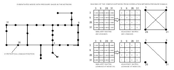Figure 1: Difference between similarity matrix, made by Pearson correlation coefficients, c_ij, and adjacency matrix, in which the value of 0 or 1 assumed by each element depends on the threshold chosen for c_ij (in the example θ = 0.990). In this case, the size of matrices is less than the number of junctions of the water distribution system, being equal to the number of installed pressure gages (indicated on the left of the figure). The hypothetical position of a leakage is also shown, together with its impact on the matrices and the resulting virtual network.

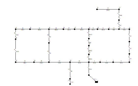Figure 2: Hanoi WDS adopted for the analyses. Link number and diameter (in mm) are indicated along the pipes.

If a leakage is formed at the i-th junction of a WDS, the total discharge Q_i(t_k) outflowing at time t_k equals the nodal demand, and can be expressed as the sum of consumer’s request and pressure-dependent water loss:

in which q_i is the average demand at node i, α(t_k) is the multiplier coefficient characterizing the demand pattern at time t_k (Figure 3), p_i(t_k) is the pressure at node i, and c and u are the leakage coefficient and the leakage exponent: they determine, respectively, the leakage entity and its dependence on the pressure (for an ideal leakage of circular shape on a steel pipe, u = 0.5).

Figure 1 (bottom right) shows the example of a leakage present at junction 28: it is easily seen that the values of the correlation coefficient in the similarity matrix decrease when the position with the leakage is involved in the calculation, giving rise to a less connected network.

The parameter adopted for the identification of the junction in which a leakage is forming is the degree centrality: the degree of a node represents the number of its nearest neighbors (in other words, the number of its connections). For an undirected network (as in this case) the column vector of node degrees’ k is given by (the symbol 1 represents an all-one column vector):

in which A is the adjacency matrix [17]. Thus, the junction in which the leak is emerging is the one characterized by the lowest correlation with respect to all the others, and the related node in the complex network has the lowest degree centrality.

4. Application to a Literature System

The methodology has been applied to the Hanoi WDS (Vietnam), since it represents a well-known literature example (Figure 2): it was introduced for the first time by [43] and then analyzed by many authors [44]. The model of the main system consists of 32 junctions and 34 pipes, organized in three loops (see [43] for the data). The numerical simulation model has been used to artificially create pressure signals at every junction of the main system, where a pressure sensor is considered to be available.

Figure 3 shows the pattern assumed for customers’ demand: its variability is typical of residential consumption, with two peaks during the day, respectively in the morning and in the evening, and a minimum during the nighttime. The time resolution adopted is 5 minutes.

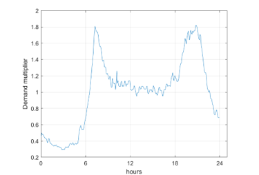Figure 3: Temporal variability of demand multiplier α(t_k) in (4), describing customers’ demand.

In Figure 3, the typical oscillations due to the stochastic nature of demand are evident. In the present paper, the simple case of uniform spatial distribution of demand pattern has been assumed. Due to the importance of correctly simulating users’ demand variability, future research will focus on such issue: to this end, the approach adopted by [45,46] appears the most suitable for real-time analyses. The time variability of pressure in the case of no leakage in the system is shown in Figure 4.

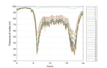Figure 4: Pressure variability over 24 hours for the junctions of Hanoi WDS.

The results have been obtained by simulations performed with Epanet software [39], with a hydraulic time step of 5 minutes and a Hazen-Williams roughness coefficient of 130 for all pipes.

The correlation between signals is evident, and may be confirmed by the plot of Figure 5, where the relationship between pairs of nodes keeping junction 2 in abscissa are shown. Similar results may be plotted for other pairs of junctions. Such behavior confirms the validity of linearity assumption between pressures

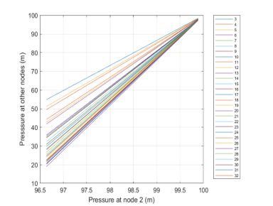Figure 5: Correlation plot for pairs of pressures between junction 2 and others

Figure 6 is a heatmap plot of the global results obtained with reference to one leakage in all possible positions, and characterized by an average outflow of 5 l/s, which may appear to be large, but actually is a relatively small value if compared to the user demand at junctions (100 l/s on average). For each column, representing an assumed position of a leakage, the figure shows the degree centrality of the nodes on a blue-tone basis, i.e., the darkest the color, the bigger is the degree of a node.

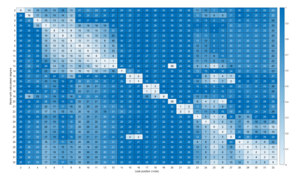Figure 6: Heatmap representation of degree centralities when varying the position of one leakage of 5 l/s in Hanoi WDS. Number in columns are the node degrees for a fixed leakage position

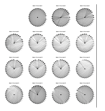Figure 7: Round plots of virtual correlation networks obtained when varying leakage position (nodes 2 to 16). The junction where the leakage is activated is drawn at the center of each plot. Thick lines are the links connecting the central node to others, while other connections are indicated with thin lines.

In this way, the lightest cell represents (for each column) the node with the least degree centrality, that is, that affected by the leakage. This is confirmed by the number indicated in each cell, giving the degree centrality. Only simulations with one leakage at a time have been considered.It is evident that, in all the cases analyzed, the node with the smallest degree is that one in which the leakage is present.

Figure 7 and Figure 8 show round plots of the virtual networks in which the node where the leakage is activated is drawn at the center. Thick lines represent the connections the central node has with others, while thin lines indicate those between other nodes.

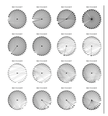Figure 8: Round plots of virtual correlation networks obtained when varying leakage position (nodes 17 to 32). The junction where the leakage is activated is drawn at the center of each plot. Thick lines are the links connecting the central node to others, while other connections are indicated with thin lines.

For each plot, the number of thick lines is the degree centrality of the node with the leakage. Such figures provide a pictorial representation of the absence of connections for the central node due to the presence of a leakage. In other words, such node is the most ‘isolated’

5. Application to a real system

In order to test the reliability of the methodology, it has been applied to the western district of Tobruk city, Libya (Figure 9, left).

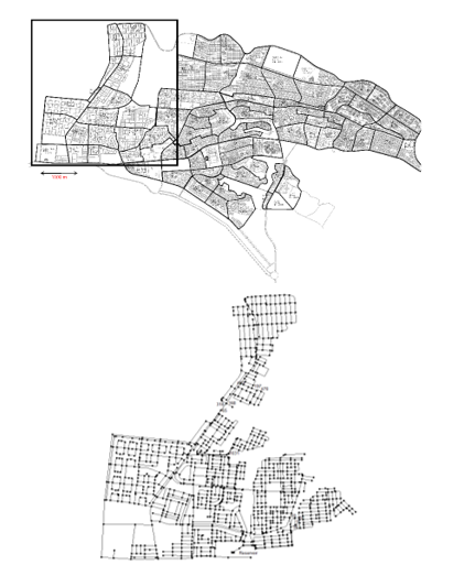Figure 9: Left: layout of the city of Tobruk (Libya), and of the western district WDS (right), where the junctions characterized by the highest frequency values reported in Figure 10 are also indicated.

It covers a surface of 8 km² and serves a population of 54600 inhabitants. The average flow supplied is 240 l/s. The model of the system includes all the details of the network, and is made of 1139 junctions and 1621 pipes (Figure 9, right).

In this case, the performance of the methodology has been evaluated as the percentage of success in identifying the junction affected by the leakage (or its neighbors, according to a predefined tolerance of 200 m, representing the average length of the pipes), varying several parameters like threshold, θ, leakage coefficient, c, and leakage exponent, u (4).

Table 1 reports the results obtained for a tolerance distance of 200 m (in other words, it is considered a good result whenever the junction with the smallest degree centrality falls within 200 meters from that in which the leakage is activated). It can be observed that, independently of the parameters assumed, the rate of success of the methodology is around 90%. This is due to the fact that there are some junctions having the minimum value of degree centrality when leakages are activated at their surroundings.

To this end, the results in terms of frequency of occurrence of the nodes have been analyzed: Figure 10 shows several cases obtained with two values of the leakage exponent (u = 0.5; 1.0) and five values for the leakage coefficient (c = 0.1,…0.5), which are typically encountered in real situations.

Table 1: Performance indicator (PI) giving the percentage of success of the methodology when applied to Tobruk WDS, with varying threshold, θ, leakage coefficient, c, and exponent, u. (The threshold number, θ, indicated as 1-10^-4 means 0.9999.)

θ	c	u	PI (%)
1-10-4	0.5	0.5	90.34
1-10-6	0.5	0.5	75.94
1-10-7	0.1	0.5	86.65
1-10-6	0.1	0.5	90.61
1-10-6	0.1	1.0	90.61
1-10-5	0.1	0.5	88.85
1-10-5	0.2	0.5	90.17
1-10-5	0.3	0.5	90.87
1-10-5	0.4	0.5	91.83
1-10-5	0.5	0.5	92.01
1-10-5	0.1	1.0	88.85
1-10-5	0.2	1.0	90.17
1-10-5	0.3	1.0	90.87
1-10-5	0.4	1.0	91.83
1-10-5	0.5	1.0	92.01

In an ideal situation, all nodes should be characterized by a frequency of one, and the frequency plots would be uniform. However, from Figure 10 it can be observed that some of them exhibit very high frequency values, indicating that their minimum degree centrality occurs not only when a leakage is present there, but also when it is activated at several other surrounding junctions. When analyzing in more detail the nodes characterized by the highest values of frequency, it can be noted that they represent particular situations of ‘bottlenecks’ of the WDS (Figure 9, right). In these cases, their minimum degree centrality hinders some other non-linear property not captured by the linear Pearson correlation coefficient, which is still under investigation.

6. Discussion and Concluding Remarks

The paper has presented the results of a new methodology introduced for the localization of leakages emerging in water distribution systems. The main advantage of the approach is that it relies only on the measurements of pressure and on cross-correlations between signals, thus avoiding the need of comparing such data with a ‘reference’ (and not well defined) scenario given by a simulation model, whose optimal calibration is generally very difficult to attain. In this paper, the simulation model has been adopted with the only purpose of generating the pressure signals.

The novelty of the research resides in the fact that it analyzes pressure measurements through Complex Networks Theory, its reliability increasing with the number of installed pressure sensors. However, the proposed approach does not represent a final solution to the problem of leakage identification, but it has to be considered a further support in the process of leakage prelocalization, that is, a fast method to assess the integrity of a WDS and, eventually, to identify areas where prompt interventions should be planned.

Two test cases have been considered: the first, representing a well-known literature system, proved the best performance of the methodology in precisely localizing the node where the leakage is emerging (which is characterized by the least degree centrality with respect to all the others); the second, a real-world network, showed a high rate of success (around 90%). The difference between the results obtained can be ascribed to the fact that, in the first case, only the main transport pipes are included in the model (in other words, the model simulates the principal ‘skeleton’ of the water distribution system). In the second case, given by a real WDS, all the pipes have been modeled, and hence the flows in the links may arrange in such a way that the conditions of minimum degree centrality do not always occur at the junction where the leakage is present, but rather in some other surrounding nodes. Actually, this is not a problem in real situations, since water managers are interested in quickly identifying the area where the leakage is forming.

Other issues still under investigations are represented by the influence on the spatial distribution of demand pattern and the presence of several reservoirs and tanks, which actually limit the performance of the methodology. In any case, the current trend in WDS management is to divide such systems in DMA (District Metered Areas), for a better control of water leakages: thus, each DMA (which is often supplied by at most one reservoir, or may be modeled in such a way through appropriate boundary conditions) can be considered as a single system and the proposed methodology applied accordingly.

The requirement of linear correlation between pressure variability is fundamental for the success of the methodology. However it is only a necessary condition, as proved by the second test case, for which the linearity in correlation is not sufficient to always guarantee the minimum degree centrality at the node with the leakage, hindering some other non-linear property not captured by the linear Pearson correlation coefficient. Also this issue is currently under investigation.

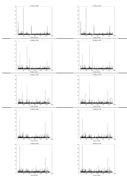Figure 10: Frequency plots of junction occurrences in minimum degree centrality when varying leakage position and for different values of leakage coefficient, c, and exponent, u. Correlation threshold of 1-10^-5 has been assumed.

Acknowledgment

The Author would like to thank the anonymous Reviewers for their comments and suggestions, which resulted in a considerable improvement of the paper.

1.  P. Swamee, A. Sharma, Design of Water Supply Pipe Networks, John Wiley & Sons, 2008.
2.  R. Beuken, C. Lavooij, A. Bosch, P. Schaap, Low leakage in the Netherlands confirmed, in Proceedings of the Water Distribution Systems Analysis Symposium 2008 (WDSA 2008), Kruger National Park, South Africa, 2008. DOI: 10.1061/40941(247)174
3.  A. Lambert, International Report: Water Losses Management and Techniques, Water Science and Technology: Water Supply, 2(4), 2002, 1–20. https://doi.org/10.2166/ws.2002.0115
4.  R.S. McKenzie, Z. Siqalaba, W. Wegelin, The State of Non-Revenue Water in South Africa; Report No. TT522/12, Water Research Commission: Lynnwood Manor, Pretoria, South Africa, 2012.
5.  A.F. Colombo, B.W. Carney, “Energy and costs of leaky pipes: toward comprehensive picture”, J. Water Resour. Plann. Manage., 128(6), 441–450, 2002. DOI: 10.1061/(ASCE)0733-9496(2002)128:6(441)
6.  M. Nicolini, Leakage Identification in Water Distribution Systems with a Complex Networks Approach, in Proceedings of the 1st IEEE International Conference on Knowledge Innovation and Invention (ICKII 2018), Jeju Island, South Korea, 2018. DOI: 10.1109/ICKII.2018.8569182
7.  J. Thornton, R. Sturm, G. Kunkel, Water Loss Control, 2nd Ed, McGraw-Hill, New York, 2008.
8.  R. Puust, Z. Kapelan, D.A. Savic, T. Koppel, “A review of methods for leakage management in pipe networks”, Urban Water Journal, 7(1), 25–45, 2010. https://doi.org/10.1080/15730621003610878
9.  M. Nicolini, L. Zovatto, “Optimal location and control of pressure reducing valves in water networks”, J. Water Resour. Plann. Manage., 135(3), 178–187, 2009. DOI: 10.1061/(ASCE)0733-9496(2009)135:3(178)H.
10.  M. Nicolini, C. Giacomello, K. Deb, “Calibration and optimal leakage management for a real water distribution network”, J. Water Resour. Plann. Manage., 137(1), 134–142, 2011. https://doi.org/10.1061/(ASCE)WR.1943-5452.0000087
11.  S. Alvisi, M. Franchini, “A procedure for the design of district metered areas in water distribution systems”, Procedia Engineering, 70, 41–50, 2014. https://doi.org/10.1016/j.proeng.2014.02.006
12.  B. Brunone, M. Ferrante, “Detecting leaks in pressurized pipes by means of transients”, J. of Hydraulic Research, 39(5), 539–547, 2001. https://doi.org/10.1080/00221686.2001.9628278
13.  D. Misiunas, J. Vitkovsky, G. Olsson, A. Simpson, M. Lambert, “Pipeline break detection using pressure transient monitoring”, J. Water Resour. Plann. Manage., 131(4), 316–325, 2005. DOI: 10.1061/(ASCE)0733-9496(2005)131:4(316)
14. M. Nicolini, A. Patriarca, Model Calibration and System Simulation from Real Time Monitoring of Water Distribution Networks, in IEEE 3rd Int.l Conf. on Computer Research and Development (ICCRD 2011), Shangai, China, 2011. DOI: 10.1109/ICCRD.2011.5763972
15.  R. Perez, V. Puig, J. Pascual, J. Quevedo, E. Landeros, A. Peralta, “Methodology for leakage isolation using pressure sensitivity analysis in water distribution networks”, Control Engineering Practice, 19(10), 1157–1167, 2011. https://doi.org/10.1016/j.conengprac.2011.06.004
16. M. V. Casillas Ponce, L. E. Garza Castañón, V. Puig Cayuela, “Model-based leak detection and location in water distribution networks considering an extended horizon analysis of pressure sensitivities”, Journal of Hydroinformatics, 16(3), 649–670, 2013. https://doi.org/10.2166/hydro.2013.019
17. D. Perfido, T. Messervey, C. Zanotti, M. Raciti, A. Costa, Automated leak detection system for the improvement of water network management, in 3rd Int.l Electronic Conf. on Sensors and Applications, 2016. https://doi.org/10.3390/ecsa-3-S5002
18.  G. Sanz, R. Perez, Z. Kapelan, D. Savic, “Leak detection and localization through demand components calibration”, J. Water Resour. Plann. Manage., 142(2), 2016. https://doi.org/10.1061/(ASCE)WR.1943-5452.0000592
19.  M.E.J. Newman, Networks: An Introduction, Oxford University Press, Oxford, 2010.
20.  A.L. Barabási, “The network takeover”, Nature Physics, 8, 14–16, 2012.
21.  R. Donner, E. Hernández-García, E. Ser-Giacomi, “Introduction to Focus Issue: Complex network perspective on flow systems”, Chaos, 27, 2017. https://doi.org/10.1063/1.4979129
22.  C. Zhou, L. Zemanová, G. Zamora-López, C. C. Hilgetag, J. Kurths, “Structure-function relationship in complex brain networks expressed by hierarchical synchronization”, New J. Phys. 9:178, 2007. doi:10.1088/1367-2630/9/6/178
23.  L. C. Carpi, P. Saco, O. Rosso, M. Gómez Ravetti, “Structural evolution of the Tropical Pacific climate network”, Eur. Phys. J. B, 85:389, 2012. DOI: 10.1140/epjb/e2012-30413-7
24.  H. Kantz, T. Schreiber, Nonlinear Time Series Analysis, 2nd Ed., Cambridge University Press, 2004.
25.  O. Giustolisi, A. Simone, L. Ridolfi, “Network structure classification and features of water distribution systems”, Water Resources Research, 53(4), 3407–3423, 2017. https://doi.org/10.1002/2016WR020071
26.  A. Yazdani, P. Jeffrey, “A complex network approach to robustness and vulnerability of spatially organized water distribution networks”. arXiv Prepr. arXiv1008.1770, 2010.
27.  A. Yazdani, R. A. Otoo, P. Jeffrey, “Resilience enhancing expansion strategies for water distribution systems: A network theory approach”, Environ. Model. Softw., 26(12), 1574–1582, 2011. DOI:10.1016/j.envsoft.2011.07.016
28.  Q. Shuang, M. Zhang, Y. Yuan, “Node vulnerability of water distribution networks under cascading failures”, Reliab. Eng. Syst. Saf., 124(C), 132–141, 2014. DOI: 10.1016/j.ress.2013.12.002
29. ] L. Berardi, R. Ugarelli, J. Rostum, O. Giustolisi, “Assessing mechanical vulnerability in water distribution networks under multiple failures”, Water Resour. Res., 50(3), 2586–2599, 2014. https://doi.org/10.1002/2013WR014770
30.  F. Chaoqi, W. Ying, W. Xiaoyang, “Research on complex networks’ repairing characteristics due to cascading failure”, Physica A, 482, 317–324, 2017. DOI: 10.1016/j.physa.2017.04.086
31.  J.A. Gutiérrez-Pérez, M. Herrera, R. Pérez-García, E. Ramos-Martínez, “Application of graph-spectral methods in the vulnerability assessment of water supply networks”, Math. Comput. Model., 57(7-8), 1853–1859, 2013. https://doi.org/10.1016/j.mcm.2011.12.008
32.  J.A. Gutiérrez-Pérez, M. Herrera, J. Izquierdo, R. Pérez-García, An approach based on ranking elements to form supply clusters in Water Supply Networks as a support to vulnerability assessment, in International Environmental Modelling and Software Society (iEMSs) Conference, Leipzig, Germany, 2012.
33. A. Yazdani, P. Jeffrey, “A note on measurement of network vulnerability under random and intentional attacks”, 2010. arXiv:1006.2791
34. N. Sheng, Y.W. Jia, Z. Xu, S.L. Ho, C.W. Kan, “A complex network based model for detecting isolated communities in water distribution networks”, Chaos, 23(4), 2013. doi: 10.1063/1.4823803
35. O. Giustolisi, L. Ridolfi, “A novel infrastructure modularity index for the segmentation of water distribution networks”, Water Resour. Res., 50(10), 7648–7661, 2014. https://doi.org/10.1002/2014WR016067
36. O. Giustolisi, L. Ridolfi, L. Berardi, “General metrics for segmenting infrastructure networks”, Journal of Hydroinformatics, 17(4), 505–517, 2015. DOI: 10.2166/hydro.2015.102
37. A. Simone, O. Giustolisi, D.B. Laucelli, “A proposal of optimal sampling design using a modularity strategy”, Water Resources Research, 52(8), 6171–6185, 2016. https://doi.org/10.1002/2016WR018944
38. R. Nazempour, M.A.S. Monfared, E. Zio, “A complex network theory approach for optimizing contamination warning sensor location in water distribution networks”, arXiv preprint arXiv:1601.02155, 2016
39. C. Giudicianni, A. Di Nardo, M. Di Natale, R. Greco, G.F. Santonastaso, A. Scala, “Topological Taxonomy of Water Distribution Networks”, Water, 10(4), 444, 1–19, 2018. https://doi.org/10.3390/w10040444
40. G.F. Santonastaso, A. Di Nardo, M. Di Natale, C. Giudicianni, R. Greco, “Scaling-Laws of Flow Entropy with Topological Metrics of Water Distribution Networks”, Entropy, 20(2), 95, 1–15, 2018. https://doi.org/10.3390/e20020095
41. L. A. Rossman, EPANET 2 Users Manual, USEPA, Cincinnati, OH, 2000.
42. E. Todini, S. Pilati, A gradient method for the analysis of pipe networks, in Int.l Conf. on Computer Applications for Water Supply and Distribution, Leicester Polytechnic, UK, 1987.
43. O. Fujiwara, D. B. Khang, “A two-phase decomposition method for optimal design of looped water distribution networks”, Water Resources Research, 26(4), 539–549, 1990. https://doi.org/10.1029/WR026i004p00539
44. A. Marchi, G. Dandy, A. Wilkins, H. Rohrlach, “A methodology for comparing evolutionary algorithms for the optimization of water distribution systems, J. Water Resour. Plann. Manage., 140(1), 786–798, 2014. https://doi.org/10.1061/(ASCE)WR.1943-5452.0000321
45.  E. Creaco, G. Pezzinga, D. Savic, “On the choice of the demand and hydraulic modeling approach to WDN real-time simulation”, Water Resources Research, 53(7), 6159–6177, 2017. https://doi.org/10.1002/2016WR020104
46. E. Creaco, E.J.M. Blokker, S.G. Buchberger, “Models for generating household water demand pulses: literature review and comparison”, J. Water Resour. Plann. Manage., 143(6), 2017. https://doi.org/10.1061/(ASCE)WR.1943-5452.0000763

(Click Here)

(Click Here)